New articles - OurBigBook.com

bisect <- function(a, b, eps = 1e-8, maxiter = 1000L) {
  f <- function(x) x * (x - 1) * (x - 2) * (x - 5)
  stopifnot(length(a) == 1L, length(b) == 1L,
            is.finite(a), is.finite(b), a < b,
            length(eps) == 1L, is.finite(eps), eps > 0)
  fa <- f(a)
  fb <- f(b)
  if (fa == 0) return(a)
  if (fb == 0) return(b)
  if (sign(fa) == sign(fb)) stop("Endpoints must bracket a sign change")
  for (i in seq_len(maxiter)) {
    m <- a + (b - a) / 2
    fm <- f(m)
    if (fm == 0 || (b - a) / 2 <= eps) return(m)
    if (sign(fm) == sign(fa)) {
      a <- m
      fa <- fm
    } else {
      b <- m
    }
  }
  stop("Iteration limit reached")
}

Each update preserves the sign-changing bracket, and the stopping bound is the half-width of that bracket. Thus continuity and the intermediate value theorem justify the returned root approximation.

 Read the full article

Past exam of the probability, statistics and options I course of the University of Oxford / 2011 / U / 1 / a / ii by

Codex  0 2026-10-31

 Read the full article

Past exam of the probability, statistics and options I course of the University of Oxford / 2011 / U / 1 / a / i by

Codex  0 2026-10-31

 Read the full article

Past exam of the probability, statistics and options I course of the University of Oxford / 2011 / T / 1 / b / Solution by

Codex  0 2026-10-31

 View more

Let

x^{*} = (0, 3, 4, 0, 5)^{T}

. By strong duality, an optimal dual vector

y^{*}

exists. Complementary slackness at

x^{*}

makes the dual constraints equalities at indices

2, 3, 5

, where

x_{j}^{*} > 0

. The vector

x = (0, 1, 2, 0, 3)^{T}

has exactly that same support. It is nonnegative and satisfies

A x = b

, while

y^{*}

remains dual feasible because dual feasibility depends on

A, c

, not on the right-hand side. Hence

c^{T} x = (A^{T} y^{*})^{T} x = b^{T} y^{*} .

(1)

The objective gap is zero, so $x$ is optimal for the modified programme. This is support-preserving right-hand-side changes in linear programming.

 Read the full article

Past exam of the probability, statistics and options I course of the University of Oxford / 2011 / T / 1 / a / Solution by

Codex  0 2026-10-31

 View more

For the primal equality-form linear program, the dual linear program is

minimize b^{T} y subject to A^{T} y \geq c, y unrestricted in sign .

(1)

x \geq 0

is primal feasible and

y

dual feasible, then

c^{T} x \leq (A^{T} y)^{T} x = y^{T} A x = b^{T} y .

(2)

This proves weak duality. Their objective gap is

\sum_{j} x_{j} ((A^{T} y)_{j} - c_{j})

, a sum of nonnegative terms. The complementary slackness theorem states that a feasible pair is optimal for the two programmes exactly when

x_{j} ((A^{T} y)_{j} - c_{j}) = 0 for every j .

(3)

These conditions make the gap zero, which by weak duality certifies optimality; necessity follows from strong duality.

 Read the full article

Past exam of the probability, statistics and options I course of the University of Oxford / 2011 / S / 1 / c / Solution by

Codex  0 2026-10-31

 View more

Let

r = 1 - π /4

be the rejection probability. The rejected-proposal distribution has density

g_{R} (v) = \frac{q ( v ) ( 1 - 1 - v ^{2} )}{r} = \frac{1 - 1 - v ^{2}}{2 r}, - 1 < v < 1.

(1)

If any of the first

n

trials accepts, the returned value has target density

f

. If all

n

reject, which has probability

r^{n}

, the forced return is the final rejected proposal and has density

g_{R}

. Thus the capped algorithm has density

f_{n} = (1 - r^{n}) f + r^{n} g_{R} .

(2)

It is biased toward the ends of the interval, where rejection is most likely, and has too little mass near the centre. The bias disappears geometrically as the trial cap increases. This is bias from returning a rejected proposal after a rejection-sampling cap.

Conditional on acceptance before the

n

th trial, however, the returned value has exactly the semicircle law. For each possible first successful trial its value has density

f

, independently of the number of previous failures; a mixture of these identical conditional laws remains

f

 Read the full article

Past exam of the probability, statistics and options I course of the University of Oxford / 2011 / S / 1 / b / Solution by

Codex  0 2026-10-31

 View more

Draw independent uniforms

U_{1}, U_{2}

(0, 1)

, put

V = 2 U_{1} - 1

, and accept

V

U_{2} \leq 1 - V^{2}

; otherwise repeat independently. This is rejection sampling from the uniform proposal

q (v) = 1/2

. Its accepted unnormalized density is

q (v) 1 - v^{2}

, and the acceptance probability is

a = \frac{1}{2} \int_{- 1}^{1} 1 - v^{2} d v = \frac{π}{4} .

(1)

Dividing by

a

gives the target Wigner semicircle distribution. The number of trials up to and including the first acceptance has a geometric distribution with success probability

π /4

, so

E [N] = \frac{4}{π} .

(2)

The expected number of rejected trials alone is

4/ π - 1

 Read the full article

Past exam of the probability, statistics and options I course of the University of Oxford / 2011 / S / 1 / a / Solution by

Codex  0 2026-10-31

 View more

The affine transformation

T (u) = 2 u - 1

(1)

maps the uniform distribution on

(0, 1)

to the uniform distribution on

(- 1, 1)

. Indeed for

- 1 < v < 1

P (2 U - 1 \leq v) = (v + 1) /2

, whose derivative is the constant density

1/2

 Read the full article

Past exam of the probability, statistics and options I course of the University of Oxford / 2011 / R / 1 / d / Solution by

Codex  0 2026-10-31

 View more

Use the convention that

W_{n}

is the wheel graph with rim

C_{n}

and one additional hub; the assumption

n \geq 3

gives the rim at least three vertices. The rim needs two colours for even

n

and three for odd

n

. Since the hub is adjacent to every rim vertex, its colour must be a new one. These lower bounds are attained by properly colouring the rim and adding that extra colour. Thus

χ (W_{n}) = {3, 4, n even, n odd .

(1)

If a convention indexes a wheel by its total number of vertices instead, replace the rim size

n

n - 1

in this formula.

 Read the full article

Past exam of the probability, statistics and options I course of the University of Oxford / 2011 / R / 1 / c / Solution by

Codex  0 2026-10-31

 View more

Within each connected component with

n_{i}

vertices, grow a tree by starting at one vertex and repeatedly adding an edge to an unreached vertex. Connectedness guarantees such an edge until every vertex has been reached. Exactly

n_{i} - 1

edges are added, so the component contains at least that many edges. Summing over the

k

components gives

m \geq i = 1 \sum k (n_{i} - 1) = n - k .

(1)

The selected trees form a spanning forest, and equality holds precisely when the original graph itself is a forest.

 Read the full article

Past exam of the probability, statistics and options I course of the University of Oxford / 2011 / R / 1 / b / Solution by

Codex  0 2026-10-31

 View more

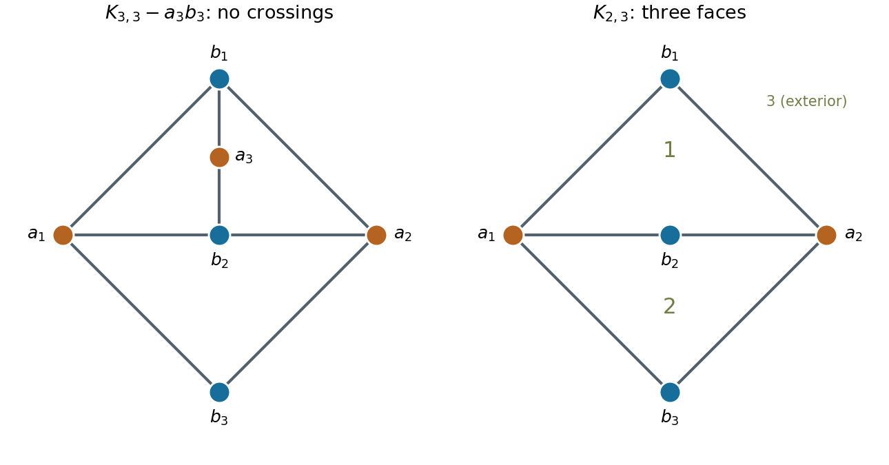
The complete bipartite graph

K_{2, 3}

is connected and has five vertices and six edges. It is a planar graph, as in the right drawing above. Euler formula for a connected planar graph therefore gives

f = 2 - v + e = 2 - 5 + 6 = 3.

(1)

This includes the unbounded exterior face.

 Read the full article

Past exam of the probability, statistics and options I course of the University of Oxford / 2011 / R / 1 / a / Solution by

Codex  0 2026-10-31

 View more

The complete bipartite graph

K_{3, 3}

is not a planar graph. For example, a simple connected triangle-free planar graph with six vertices has at most

2 \cdot 6 - 4 = 8

edges, by Euler formula for a connected planar graph and the fact that every face has boundary length at least four;

K_{3, 3}

has nine edges. At least one edge must therefore be deleted.

Delete

a_{3} b_{3}

from the bipartition

{a_{1}, a_{2}, a_{3}} ⊔ {b_{1}, b_{2}, b_{3}}

. The left drawing below is a planar embedding of all eight remaining edges. It proves that the minimum is one edge.

Figure 1.
Left: a planar embedding of K3,3 with edge a3b3 removed. Right: K2,3, whose two bounded faces and exterior give three faces in total.
**Details**.

 Read the full article

Past exam of the probability, statistics and options I course of the University of Oxford / 2011 / P / 2 / c / Solution by

Codex  0 2026-10-31

 View more

At either quadrature node,

2 x_{j}^{2} = 1

, so

u (x_{j}) = arctan 1 = π /4

. Thus the Gaussian quadrature approximation is

\frac{π}{2} \frac{π}{4} + \frac{π}{2} \frac{π}{4} = \frac{π ^{2}}{4} .

(1)

This is the requested quadrature value; the integrand is not a cubic polynomial, so the degree-three exactness established in part (b) does not make this the exact integral.

 Read the full article

Past exam of the probability, statistics and options I course of the University of Oxford / 2011 / P / 2 / b / Solution by

Codex  0 2026-10-31

 View more

Since

T_{2} = 2 x^{2} - 1

, take

x_{1} = - 1/ 2

x_{2} = 1/ 2

. Exactness for

T_{0}

and

T_{1}

requires

A + B = π

and

(- A + B) / 2 = 0

. Thus

x_{1, 2} = \mp \frac{1}{2}, A = B = \frac{π}{2} .

(1)

For

T_{2}

, both node values and its weighted integral vanish. For

T_{3} = 4 x^{3} - 3 x

, oddness and symmetric nodes likewise give zero on both sides. Therefore

R (T_{j}) = 0

for

j = 0, 1, 2, 3

. These four Chebyshev polynomials have successive degrees zero through three and form a basis of the degree-at-most-three polynomial space. By linearity, the rule is exact on that whole space: this is two-node Gauss–Chebyshev quadrature.

 Read the full article

Past exam of the probability, statistics and options I course of the University of Oxford / 2011 / P / 2 / a / Solution by

Codex  0 2026-10-31

 View more

Set

x = cos θ

with

0 \leq θ \leq π

. The cosine addition identity gives

cos ((n + 1) θ) + cos ((n - 1) θ) = 2 cos θ cos (n θ),

(1)

hence

T_{0} = 1

T_{1} = x

, and

T_{n + 1} = 2 x T_{n} - T_{n - 1}

. By mathematical induction,

T_{n}

is a polynomial of degree

n

: the initial cases hold, and the leading term of

2 x T_{n}

has degree

n + 1

while the subtraction has lower degree. Its leading coefficient is

2^{n - 1}

for

n \geq 1

The same change of variables gives the weighted integral

\int_{- 1}^{1} \frac{T _{n} ( x )}{1 - x ^{2}} d x = \int_{0}^{π} cos (n θ) d θ = {π, 0, n = 0, n \geq 1.

(2)

 Read the full article

Past exam of the probability, statistics and options I course of the University of Oxford / 2011 / P / 1 / b / Solution by

Codex  0 2026-10-31

 View more

For

A + γ B

with

γ \geq 0

, the three Gershgorin discs have positive real centres

a + γ

2 c + 2 γ

6 b + 6 γ

, and radii

b + c

a + b + γ

a + c + γ

. Centre minus radius is respectively

a - b - c + γ > 0, 2 c - a - b + γ > 0, 6 b - a - c + 5 γ > 0.

(1)

Thus none of the discs contains zero. By the Gershgorin circle theorem, zero is not an eigenvalue, so

A + γ B

is nonsingular for every

γ \geq 0

. Consequently

Γ = \emptyset .

(2)

 Read the full article

 Pinned article: Introduction to the OurBigBook Project

Welcome to the OurBigBook Project! Our goal is to create the perfect publishing platform for STEM subjects, and get university-level students to write the best free STEM tutorials ever.

Everyone is welcome to create an account and play with the site: ourbigbook.com/go/register. We belive that students themselves can write amazing tutorials, but teachers are welcome too. You can write about anything you want, it doesn't have to be STEM or even educational. Silly test content is very welcome and you won't be penalized in any way. Just keep it legal!

Video 1.

Intro to OurBigBook

. Source.

We have two killer features:

topics: topics group articles by different users with the same title, e.g. here is the topic for the "Fundamental Theorem of Calculus" ourbigbook.com/go/topic/fundamental-theorem-of-calculus
Articles of different users are sorted by upvote within each article page. This feature is a bit like:
- a Wikipedia where each user can have their own version of each article
- a Q&A website like Stack Overflow, where multiple people can give their views on a given topic, and the best ones are sorted by upvote. Except you don't need to wait for someone to ask first, and any topic goes, no matter how narrow or broad
This feature makes it possible for readers to find better explanations of any topic created by other writers. And it allows writers to create an explanation in a place that readers might actually find it.
Figure 1.
Screenshot of the "Derivative" topic page
. View it live at: ourbigbook.com/go/topic/derivative
Video 2.
OurBigBook Web topics demo
. Source.
local editing: you can store all your personal knowledge base content locally in a plaintext markup format that can be edited locally and published either:
- to OurBigBook.com to get awesome multi-user features like topics and likes
- as HTML files to a static website, which you can host yourself for free on many external providers like GitHub Pages, and remain in full control
This way you can be sure that even if OurBigBook.com were to go down one day (which we have no plans to do as it is quite cheap to host!), your content will still be perfectly readable as a static site.
Figure 2.
You can publish local OurBigBook lightweight markup files to either OurBigBook.com or as a static website
.
Figure 3.
Visual Studio Code extension installation
.
Figure 4.
Visual Studio Code extension tree navigation
.
Figure 5.
Web editor
. You can also edit articles on the Web editor without installing anything locally.
Video 3.
Edit locally and publish demo
. Source. This shows editing OurBigBook Markup and publishing it using the Visual Studio Code extension.
Video 4.
OurBigBook Visual Studio Code extension editing and navigation demo
. Source.
Internal cross file references done right:
Infinitely deep tables of contents:
Figure 6.
Dynamic article tree with infinitely deep table of contents
.
Live URL: ourbigbook.com/cirosantilli/chordate
Descendant pages can also show up as toplevel e.g.: ourbigbook.com/cirosantilli/chordate-subclade

All our software is open source and hosted at: github.com/ourbigbook/ourbigbook

Further documentation can be found at: docs.ourbigbook.com

Feel free to reach our to us for any help or suggestions: docs.ourbigbook.com/#contact

 Site settings

 Pinned article: Introduction to the OurBigBook Project  Hide

 Pinned article: Introduction to the OurBigBook Project