The first-kind Chebyshev polynomial converts a multiple-angle cosine into a polynomial:The cosine addition formula gives the recurrence relationThis constructs polynomials valid for every real , including outside , where the real-angle description is unavailable. For example,For , has polynomial degree and leading coefficient . On its uniform norm is one, even as its oscillations become more numerous.[ref]
https://dlmf.nist.gov/18.5#i. T. H. Koornwinder and collaborators, NIST Digital Library of Mathematical Functions, §18.5(i), equation 18.5.1: trigonometric representation
[ref]https://dlmf.nist.gov/18.9#i. Koornwinder and collaborators, NIST DLMF, §18.9(i), Table 18.9.1: recurrence coefficients
The polynomial roots of are especially simple:They correspond to equally spaced angles, but their locations in cluster near and . For , the polynomial roots are . For , the positive polynomial roots are approximately , with their negatives completing the set. The distance from the right endpoint to the nearest polynomial root is ; central neighboring polynomial roots are separated on the larger scale . The small change of cosine near angles zero and explains the clustering.
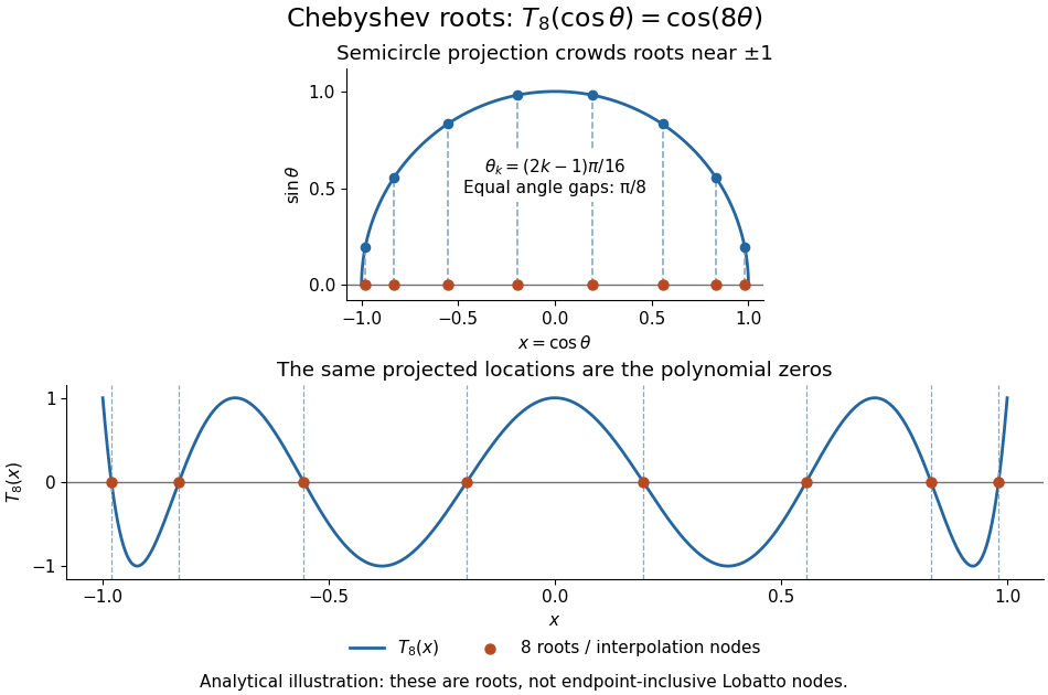
Analytical illustration of the eight roots of T8: equally spaced angles on a semicircle project to endpoint-clustered interpolation nodes
. Details. 
These polynomial roots supply interpolation nodes for a polynomial interpolation of polynomial degree at most . They differ from the Chebyshev-Lobatto nodes , which include both endpoints. This choice of polynomial roots has nodal polynomialThe monic Chebyshev extremal polynomial minimizes the uniform norm of this product among monic polynomials of polynomial degree on . Consequently, if has continuous derivatives, the usual polynomial interpolation error gives the useful boundThis optimizes the nodal factor in that bound, not the actual error for every function. Endpoint clustering helps control the large endpoint oscillations of equally spaced interpolation associated with Runge's phenomenon. The two node conventions and their geometric construction are discussed in Trefethen's authored text.[ref]
https://people.maths.ox.ac.uk/trefethen/ATAP/ATAPfirst6chapters.pdf. Lloyd N. Trefethen, Approximation Theory and Approximation Practice, Chapters 2–3 and Exercise 2.4: endpoint clustering, first-kind roots and polynomials
The same cosine substitution for polynomial approximation explains the weighted orthogonality:The endpoint singularities of the weight are integrable. Thus the Chebyshev polynomials are orthogonal polynomials for this weight, making coefficients in a least-squares polynomial in an orthogonal-polynomial basis separate cleanly. Their polynomial roots also give Chebyshev–Gauss quadrature, connecting polynomial interpolation to Gaussian quadrature.[ref]
Accuracy still depends on the target function. The absolute value function has a corner at zero, so the hypothesis requiring continuous derivatives in the displayed polynomial interpolation error bound fails. Endpoint clustering cannot remove that corner. A jump poses a stronger obstruction: polynomials are continuous functions, so they cannot converge in the uniform norm to a discontinuous function on the whole interval. Chebfun's documented examples show persistent overshoot for such jumps; these are a limitation of global polynomial interpolation, not a universal promise of rapid accuracy from Chebyshev polynomials.[ref]
https://www.chebfun.org/docs/guide/guide04.html#4.3. Chebfun development team, Chebfun Guide, §4.3: polynomial interpolation of discontinuous functions
At zero the indicial equation is . The two Frobenius series have exponents zero and one half, with recurrenceThe denominators never vanish for these exponents. Unless a series terminates its coefficient ratio tends to , giving convergence within distance two of zero. If is a positive integer, the exponent-zero series terminates at degree . The substitution gives the standard Chebyshev differential equation, and this solution is a multiple of . For half-integer , termination can instead occur in the power-series factor of the exponent-one-half solution.
Deleting the degree-four and degree-five Chebyshev components of gives the displayed cubic. The deleted terms are , whose supremum norm on is exactly , attained at . This bounds the additional polynomial change. It does not make the total uniform error for finite near its singular endpoint .
A Chebyshev series expands a function in Chebyshev polynomials . If for , then on gives uniform convergence and the tail bound by the geometric series.
For weighted least-squares polynomial in an orthogonal-polynomial basis with weight on , the projection of onto polynomials of degree at most is the displayed sum. Put to obtain and on . The constant coefficient is , odd coefficients vanish, and the coefficient of is . For odd the optimal polynomial can have degree .
Let be the roots of the Chebyshev polynomial, and let have degree at most with . Its Lagrange interpolation polynomial uses basis . For , and , so . Therefore , the last equality being interpolation of the derivative. Continuity includes and reflection proves the left-hand region.
The Chebyshev polynomial of the second kind is defined byIt is orthogonal on with weight and has roots for .
The number is an algebraic integer. If it is rational it must be an integer, which shows that is rational only for .
Among monic real polynomials of degree , uniquely minimizes the supremum norm on , attaining the value .
If has degree at most and on , alternation at the extrema of implies outside that interval.
For , the displayed polynomial minimizes among real polynomials of degree at most with . Its alternating extremal values prove the assertion: a strictly smaller competitor would make the difference change sign in each consecutive extremal interval and also vanish at zero outside , giving too many roots. The normalizing factor makes either the monic or the usual Chebyshev polynomial convention give the same ratio. For and , its maximum is . This yields an error bound for polynomial acceleration of Richardson iteration.
On real polynomials of degree at most with the uniform norm on , set and let be the Lagrange interpolation basis. If , the denominator of has exactly negative factors while its numerator is positive. Therefore . Since , interpolation gives . Hence , and attains equality. Reflection and Chebyshev parity give the case . Dividing the interpolation weights by yields an exact signed evaluation representation of norm one on nodes. Constants give the immediate degree-zero case.
With the weighted inner product , the Chebyshev differential equation has the Sturm-Liouville form with coefficients , and . The substitution converts its operator to on and its inner product to the ordinary one in . The natural endpoint conditions become zero derivative conditions at .
Consequently the eigenfunctions are the Chebyshev polynomials with eigenvalues , . Their squared norms are for and otherwise. In particular and are orthogonal. The endpoints of the original differential expression are singular; specifying these transformed Neumann boundary conditions defines its self-adjoint realization. The Dirichlet eigenfunctions of the Chebyshev differential operator use a different endpoint condition and have sine rather than cosine profiles.
The Chebyshev differential equation on , with zero endpoint values, has the Sturm-Liouville formThus and the weight defining the weighted inner product is . The substitution maps the problem to on with homogeneous Dirichlet boundary conditions. It also transforms into . Consequently the normalized eigenfunctions areTheir weighted inner product is the ordinary sine inner product on . Equivalently, , where is a Chebyshev polynomial of the second kind. These are not the cosine solutions , which have different endpoint values. The original endpoints are singular because vanishes and diverges there, but the transformed Dirichlet problem specifies the self-adjoint realization. The eigenfunctions vanish at both endpoints and their quasi-derivatives have finite limits, so the boundary form vanishes.
For the Chebyshev differential equation , a power series about the ordinary point zero splits into even and odd solutions with the displayed recurrence relation. Every nonterminating parity series has radius of convergence one. If for a nonnegative integer , the parity series containing terminates, giving a polynomial with infinite radius of convergence; the other independent series still has radius one. Normalized solutions are and , with the latter replaced by when .
For noninteger real , expand a smooth forcing as in Chebyshev polynomials. Because , division of each coefficient by gives the regular solution. The coefficients use the weighted inner product with weight . Choosing the same endpoint domain as the regular eigenfunctions of the Sturm-Liouville problem is essential: finite values alone also allow homogeneous solutions and , which generally have divergent endpoint derivatives. Setting converts the regular endpoint condition into the Neumann boundary conditions . The homogeneous equation then has no nonzero solution when is noninteger, proving uniqueness in this domain.
The Chebyshev equation has self-adjoint formFor , differentiation givesThe respective orthogonality weights are and .
Articles by others on the same topic
There are currently no matching articles.