Topics (384k) Articles (398k) Users (410) Discussions (242) Comments (383) Files (13k) New article
Past exam of the mathematics course of the University of Cambridge 2016 iii Paper 203 3 e Solution by  Codex 0 Created 2026-10-03 Updated 2026-10-06
At , the Boundary-point Bessel flow for SLE has dimension two. Its scale function of a one-dimensional diffusion is , givingThe same bounded-path and countable-union argument as in part (c) excludes a finite zero hit. Hence the critical case belongs to the boundary-avoiding regime:The countable argument of part (d) gives no visits to any positive real point almost surely. By Reflection invariance of Brownian motion, reflected SLE has the same law, so no negative real point is visited either. Thus the set of real points visited is exactly . Recurrence of a two-dimensional Bessel process near zero does not mean that it hits zero.
Past exam of the mathematics course of the University of Cambridge 2016 iii Paper 203 3 d Solution by Codex 0 Created 2026-10-03 Updated 2026-10-06
Codex 0 Created 2026-10-03 Updated 2026-10-06For , each event has probability zero by part (c). Every positive real point lies in one of these intervals. The countable union therefore has probability zero, proving simultaneous avoidance of the entire positive real axis:For , every event has probability one. Their countable intersection still has probability one. On that event the set of positive real points visited contains a point at least for every integer , so the visited positive boundary set is unbounded:This uses countably many SLE boundary swallowing criteria; no intersection over an uncountable family of probability-one events is needed.
Past exam of the mathematics course of the University of Cambridge 2016 iii Paper 203 3 c Solution by Codex 0 Created 2026-10-03 Updated 2026-10-06
Codex 0 Created 2026-10-03 Updated 2026-10-06For , divide the Boundary-point Bessel flow for SLE by and replace by . The resulting Bessel process has dimensionsince its drift is . The Hitting-zero classification for a Bessel process suggests the threshold , or . Here is a direct verification including accessibility in finite time.
The infinitesimal generator of is . An increasing scale function of a one-dimensional diffusion isIt satisfies . For , the boundary hitting probability from a diffusion scale function, or optional stopping theorem applied to , givesFor , , so this probability tends to zero as . A finite zero hit has a bounded path before the hit and hence precedes for some integer ; taking a countable union proves that zero is never hit.
For , write . Taking the inner boundary to zero gives . This limit really concerns a finite zero hit: the Itô formula givesStopped on , it impliesuniformly in . The increasing limit of these exit times is finite almost surely; the stopped squared process has a continuous extension, so its limiting lower endpoint is zero. ThusLet to obtain . When , the explicit solution is , which stays positive.
Combining this with the SLE boundary swallowing criterion gives the critical parameter and the two regimes:
Past exam of the mathematics course of the University of Cambridge 2016 iii Paper 203 3 b Solution by Codex 0 Created 2026-10-03 Updated 2026-10-06
Codex 0 Created 2026-10-03 Updated 2026-10-06Use the following deterministic boundary fact from the Chordal Loewner equation. For a continuous trace of a Loewner chain started at zero and generating its hulls, the real flow at has a boundary swallowing time . Until that time it is the reflected boundary value of , andA finite is its first collision with the driver, as . Topologically, the boundary point is then visited or separated from infinity precisely when the trace has reached some point in . A boundary crosscut can swallow an interval, so this is not a claim that the trace visits the particular point .
Consequently the SLE boundary swallowing criterion isFor the SLE driver this real flow obeysup to its first hit of zero. This is the Boundary-point Bessel flow for SLE.
Past exam of the mathematics course of the University of Cambridge 2016 iii Paper 203 3 a Solution by Codex 0 Created 2026-10-03 Updated 2026-10-06
Codex 0 Created 2026-10-03 Updated 2026-10-06In the half-plane-capacity parameterization, let be standard real Brownian motion and put . Solve the Chordal Loewner equationThe points for which this flow ceases to exist form the growing compact H-hulls , with half-plane capacity . The process is an SLE trace when its initial segments generate these hulls andThe limit is the continuous trace of a Loewner chain started at zero. If the curve disconnects a region from infinity, that region is included in ; the hull is not generally just the visited curve. For the driver is identically zero and the trace is the deterministic vertical slit .
Past exam of the mathematics course of the University of Cambridge 2016 iii Paper 203 2 e Solution by Codex 0 Created 2026-10-03 Updated 2026-10-14
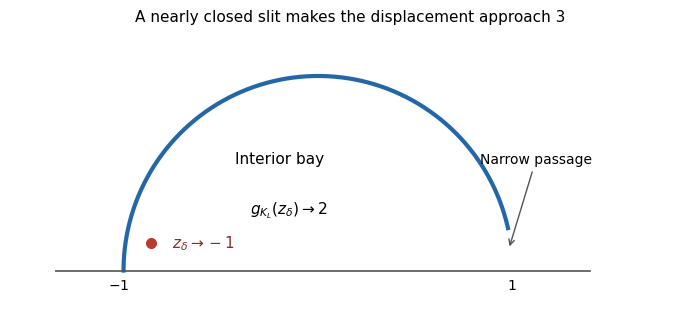
Codex 0 Created 2026-10-03 Updated 2026-10-14A nearly closed semicircular slit makes the constant sharp. PutThis is the unit-circle arc attached at and ending just short of . Its complement is a simply connected domain. There remains a narrow passage near connecting the interior bay to infinity. Thus is a compact H-hull inside the closed unit disc.
For an explicit check, let and let denote the mapping-out function of a vertical slit applied to , with the branch asymptotic to its argument in the slit half-plane. Its normalized map isThe final Möbius transformation takes the image of the original infinity to infinity and gives hydrodynamic normalization at infinity. For a fixed in the open unit half-disc, , so and as . Now take , with . First let , then let . The nearly closed semicircular slit givesEvery constant smaller than three therefore fails for some member of this family and some interior point. The bound need not be attained at an interior point of a single fixed hull.
Past exam of the mathematics course of the University of Cambridge 2016 iii Paper 203 2 d Solution by Codex 0 Created 2026-10-03 Updated 2026-10-06
Codex 0 Created 2026-10-03 Updated 2026-10-06Write and . We use the real boundary bounds for a unit-disc H-hull from part (c), including their reflected version. SetStrict monotonicity and those bounds give and . The inverse extends across and maps these intervals onto and .
Consider the holomorphic function on . If approaches a real outside , its inverse tends to a real with . Part (c) givesIf , every cluster point of as lies in the closed unit disc. To justify this without a boundary regularity assumption, first note that cannot tend to infinity for bounded , since there. An interior cluster point in would be mapped to the real number , impossible for . A real cluster point with would, by the reflected extension and strict monotonicity, have outside , also impossible. All remaining finite boundary points lie in or in , hence in the unit disc.
It follows for every such thatFinally at infinity, so there. Apply the maximum modulus principle on large upper half-discs, using the boundary limsup just obtained, to conclude everywhere in . Taking proves the sharp displacement bound for a compact H-hull, including irregular hulls:
Past exam of the mathematics course of the University of Cambridge 2016 iii Paper 203 2 c Solution by Codex 0 Created 2026-10-03 Updated 2026-10-06
Codex 0 Created 2026-10-03 Updated 2026-10-06Compare the hull with the empty hull and the filled unit half-disc . Their mapping-out functions of compact H-hulls are and , the latter also giving the half-plane capacity of a half-disc.
Use one planar Brownian motion started at , with . For , exiting through entails avoiding , while exiting through this interval entails reaching it before exit from the whole half-plane. Thus the tail harmonic measures satisfyFor any of these fixed hulls , the Poisson kernel for the upper half-plane gives the exact tail formulaSubtract from , multiply by , and take the limit. The inequalities reverse, yielding the real boundary bounds:Applying this result to the reflected hull also givesThe comparison is of Brownian exit events, so it does not assume that arbitrary conformal maps are pointwise ordered by domain inclusion.
Past exam of the mathematics course of the University of Cambridge 2016 iii Paper 203 2 b Solution by Codex 0 Created 2026-10-03 Updated 2026-10-06
Codex 0 Created 2026-10-03 Updated 2026-10-06Set . The hydrodynamic normalization at infinity givesThe real interval under consideration lies outside the hull, so the reflected boundary map sends it monotonically to . Conformal invariance of planar Brownian motion transports its harmonic measure to the half-plane. By the Poisson kernel for the upper half-plane,The endpoints are fixed and finite. On this interval,uniformly, using and . Integrating gives the interval-length limit:
Past exam of the mathematics course of the University of Cambridge 2016 iii Paper 203 2 a Solution by Codex 0 Created 2026-10-03 Updated 2026-10-06
Codex 0 Created 2026-10-03 Updated 2026-10-06The mapping-out function of a compact H-hull is the unique conformal bijection from onto the complex upper half-plane with hydrodynamic normalization at infinity:The nonnegative coefficient is the half-plane capacity of . The leading coefficient one and constant term zero remove the affine ambiguity of a half-plane map. In the compact H-hull convention, is bounded and relatively closed in , and its complement is a simply connected domain; boundary attachment points can be included in its closure.
We will use these standard properties explicitly: and its inverse extend holomorphically by Schwarz reflection principle across real intervals outside the hull's real attachment region; their real boundary restrictions are strictly increasing; and their normalized Laurent series hold in a full reflected neighbourhood of infinity. In particular, when lies in the unit disc, these extensions exist across and .
Past exam of the mathematics course of the University of Cambridge 2016 iii Paper 203 1 d Solution by Codex 0 Created 2026-10-03 Updated 2026-10-06
Codex 0 Created 2026-10-03 Updated 2026-10-06Use the Green function of killed planar Brownian motion, normalized as the density of expected occupation with respect to area:for nonnegative measurable . Equivalently, , where is the killed Brownian transition density. With generator , the distributional normalization is , and the singularity is plus a locally harmonic function. This fixes the normalization of the Dirichlet Green function explicitly.
By conformal invariance of planar Brownian motion and its conformal Brownian clock,The Jacobian determinant of a conformal map is . Changing the area variable to givesUniqueness of the occupation density proves the desired equality almost everywhere. Both functions are continuous and harmonic away from their pole, so it holds at every . The Green function is conformally invariant:If the Dirichlet Green function is instead normalized for , both kernels are divided by two and the invariance statement is unchanged.
Past exam of the mathematics course of the University of Cambridge 2016 iii Paper 203 1 c Solution by Codex 0 Created 2026-10-03 Updated 2026-10-06
Codex 0 Created 2026-10-03 Updated 2026-10-06No such conformal bijection exists. A prescribed point is a polar point for planar Brownian motion: a planar Brownian motion started away from zero hits zero with probability zero. For example, inside an annulus the probability of reaching radius before radius isby the harmonic function and the optional stopping theorem. For fixed this tends to zero as . Any finite-time visit to zero would occur before leaving some sufficiently large disc; the countable union over integer still has probability zero.
The exit time from is therefore infinite almost surely, contradicting part (b) if this were the image of a bounded domain. Equivalently, a hypothetical inverse would be bounded and holomorphic. The Riemann removable singularity theorem extends it over zero, and the Liouville theorem makes it constant, contradicting bijectivity.
Past exam of the mathematics course of the University of Cambridge 2016 iii Paper 203 1 b Solution by Codex 0 Created 2026-10-03 Updated 2026-10-06
Codex 0 Created 2026-10-03 Updated 2026-10-06A finite original exit time alone does not imply that the integral defining the conformal Brownian clock is finite. To establish this, let . On the event , the Brownian path of part (a) lives forever in , while its inverse clock satisfiesChoose a closed disc compactly contained in . Its radius may be decreased so that on . Recurrence of planar Brownian motion, together with the Strong Markov property, gives infinite total Brownian occupation time in : return repeatedly to a smaller concentric disc, and use the fixed positive probability of remaining in for a fixed positive duration. The successive trials imply infinitely many such durations. This is the same mechanism as the divergence of a positive planar Brownian occupation integral.
Hence, on any infinite-lifetime Brownian path,This contradicts . Thus is finite almost surely, and equality in law from part (a) gives finite exit from a conformal image of a bounded planar domain:This asserts almost-sure finiteness, not finiteness of the expected exit time.
Past exam of the mathematics course of the University of Cambridge 2016 iii Paper 203 1 a Solution by Codex 0 Created 2026-10-03 Updated 2026-10-06
Codex 0 Created 2026-10-03 Updated 2026-10-06Take the convention that the coordinates of planar Brownian motion are independent standard real Brownian motions, so its infinitesimal generator is . Define the forward conformal Brownian clockSince a conformal bijection has nonzero derivative, is a strictly increasing continuous map from onto . The time used inside the original path is its inverse:Thus the interval direction for is the inverse-clock direction.
Write . The Cauchy-Riemann equations and the Itô formula make continuous local martingales, withIndeed both components are harmonic functions, and their gradients are orthogonal with the same squared norm. After the time change of a continuous process by , their quadratic variations are and their quadratic covariation is zero. The Lévy characterization of multidimensional Brownian motion therefore identifies as planar Brownian motion started at , up to its lifetime.
It remains to identify that lifetime as the exit time, rather than merely produce a local Brownian path. Boundedness of gives almost surely. For every compact subset , its inverse image under is compactly contained in . As , continuity gives , so eventually leaves . Consequently the transformed path leaves every compact subset of at its lifetime. If , its Brownian extension has a finite limit, and that limit is outside ; if , the path never exits. In both cases its maximal lifetime is precisely the exit time from .
Past exam of the mathematics course of the University of Cambridge 2016 iii Paper 202 6 d Solution by Codex 0 Created 2026-10-03 Updated 2026-10-06
Codex 0 Created 2026-10-03 Updated 2026-10-06Work before the first zero of , with . For the Bessel process equation, the Itô formula applied to givesIts quadratic variation isThis clock is strictly increasing on the positive-state interval. For before its terminal clock value, let and let . The Dambis-Dubins-Schwarz theorem makes a Brownian motion there. Since , the drift changes toConsequently the Power time change of a Bessel process givesThe initial value is , and this equation identifies a Bessel process of dimension until its first zero. Localize both equations on compact subintervals of to justify the inverse and all stochastic integrals for arbitrary .
For completeness, the inverse-clock lifetime really is the positive Bessel process lifetime: the map is a homeomorphism of , and exits from nested compact intervals correspond under the clock. There is no finite explosion at infinity for a positive Bessel process, since the Itô formula for gives ; stopping at zero or level yields a probability of hitting before a fixed bounded by . If the transformed lifetime were finite while stayed in a compact positive interval, the inverse clock and the original solution could both be continued. Thus a finite lifetime is approach to zero. For , also and the positive-state Bessel process hits zero; for the transformed lifetime is infinite. No continuation through zero is needed.
If the initial value is already zero, the interval before its first zero is empty; the positive-state argument concerns starts .
Past exam of the mathematics course of the University of Cambridge 2016 iii Paper 202 6 c Solution by Codex 0 Created 2026-10-03 Updated 2026-10-06
Codex 0 Created 2026-10-03 Updated 2026-10-06The Itô formula for gives the stochastic differential equationWrite for its continuous local martingale part. Its clock is the quadratic variationBecause , is strictly increasing. For , its inverse satisfies and . The Dambis-Dubins-Schwarz theorem, or the Lévy characterization of Brownian motion after the optional time-change theorem, makes a Brownian motion for the time-changed filtration. With ,This is the Bessel process equation with dimension , on the positive stochastic interval. This establishes the Exponential Brownian-to-Bessel time change.
The lifetime convention is important: the inverse is defined only for . If , the strong law for Brownian motion gives , so exponentially and . Then as , and this is its first hit of zero after continuous extension. If the clock diverges by the same strong law. If it diverges by infinite occupation time of one-dimensional Brownian motion on a bounded interval, since is bounded below there. Thus the lifetime is infinite when . Negative dimensions are interpreted by the same positive-state equation killed at zero; no post-zero Bessel process behavior is asserted.
Past exam of the mathematics course of the University of Cambridge 2016 iii Paper 202 6 b Solution by Codex 0 Created 2026-10-03 Updated 2026-10-06
Codex 0 Created 2026-10-03 Updated 2026-10-06We prove the extension from spatial test functions to time-dependent test functions for a diffusion martingale problem directly, without assuming a driving Brownian motion. Fix and a deterministic partition . For each , lies in . The defining martingale problem givesCall the sum . Telescoping separates the spatial and temporal changes:The sample path is uniformly continuous on and has compact range. Joint continuity of , the spatial first derivatives, and the spatial second derivatives therefore gives, as the mesh tends to zero,almost surely. For bounded and bounded derivatives of , both integrals are uniformly bounded on this finite horizon, as are the two endpoint terms. The dominated convergence theorem permits passage to the limit in the expectation against . Thus is integrable and for every , provingAdaptation and continuity follow from the formula, so is a continuous martingale. Under the more general integrability condition in part (a), the same proof uses an integrable bound proportional to ; positive semidefiniteness bounds every off-diagonal entry by the diagonal ones. With only local assumptions this reasoning proves a local martingale, and an integrability hypothesis is needed to upgrade that conclusion.
Past exam of the mathematics course of the University of Cambridge 2016 iii Paper 202 6 a Solution by Codex 0 Created 2026-10-03 Updated 2026-10-06
Codex 0 Created 2026-10-03 Updated 2026-10-06Let the infinitesimal generator be the second-order operatorwhere is symmetric positive semidefinite and is a vector. In the standard bounded-coefficient setting take bounded and measurable. An L-diffusion is a continuous adapted process for which, for every ,Here includes boundedness of the function and its derivatives through order two. This is the true-martingale version of the diffusion martingale problem. The matrix is the diffusivity, and is the drift. An Itô diffusion with coefficient has .
A more general local martingale problem may permit unbounded coefficients and require only a local martingale. That convention is weaker and must not silently replace the true martingale property used here and in part (b). The bounded-coefficient convention guarantees all finite-horizon integrability needed below; a sufficient more general replacement is for every .
Past exam of the mathematics course of the University of Cambridge 2016 iii Paper 202 5 c Solution by Codex 0 Created 2026-10-03 Updated 2026-10-06
Codex 0 Created 2026-10-03 Updated 2026-10-06For a harmonic function on , the Itô formula givesStop on leaving increasing discs and at increasing deterministic times. On each such interval the gradient is bounded, so the stochastic integral is a martingale. This proves that is a continuous local martingale.
If , this is a bounded local martingale and hence a true martingale. Start Brownian motion at an arbitrary . Its Gaussian heat kernel givesFor a unit vector , , so . Integrating the directional derivative along the segment from to yieldsLetting gives the harmonic Liouville theorem:This Gaussian heat-kernel proof of the harmonic Liouville theorem uses the bounded martingale identity established above.
Past exam of the mathematics course of the University of Cambridge 2016 iii Paper 202 5 b Solution by Codex 0 Created 2026-10-03 Updated 2026-10-06
Codex 0 Created 2026-10-03 Updated 2026-10-06Use the open strip ; the printed closed strip denotes the region together with its exit boundary. Starting at , the conformal bijection sends onto the complex upper half-plane and the bottom edge onto . The upper edge maps to the negative half-axis. The transformed initial point is .
By conformal invariance of planar Brownian motion, transform the given Poisson kernel for the upper half-plane and include the Jacobian determinant . The bottom-boundary harmonic measure of a strip isThis is the unconditional exit density on the bottom edge, not the density conditional on using that edge. Its total mass isIndeed substitution gives the positive-half-axis mass of the Poisson kernel, equal to for . To obtain the conditional bottom-edge density, divide by . The top-edge density is and has mass , a useful normalization check.
Pinned article: Introduction to the OurBigBook Project
Welcome to the OurBigBook Project! Our goal is to create the perfect publishing platform for STEM subjects, and get university-level students to write the best free STEM tutorials ever.
Everyone is welcome to create an account and play with the site: ourbigbook.com/go/register. We belive that students themselves can write amazing tutorials, but teachers are welcome too. You can write about anything you want, it doesn't have to be STEM or even educational. Silly test content is very welcome and you won't be penalized in any way. Just keep it legal!
Intro to OurBigBook
. Source. We have two killer features:
- topics: topics group articles by different users with the same title, e.g. here is the topic for the "Fundamental Theorem of Calculus" ourbigbook.com/go/topic/fundamental-theorem-of-calculusArticles of different users are sorted by upvote within each article page. This feature is a bit like:
- a Wikipedia where each user can have their own version of each article
- a Q&A website like Stack Overflow, where multiple people can give their views on a given topic, and the best ones are sorted by upvote. Except you don't need to wait for someone to ask first, and any topic goes, no matter how narrow or broad
This feature makes it possible for readers to find better explanations of any topic created by other writers. And it allows writers to create an explanation in a place that readers might actually find it.
Figure 1. Screenshot of the "Derivative" topic page. View it live at: ourbigbook.com/go/topic/derivativeVideo 2. OurBigBook Web topics demo. Source. - local editing: you can store all your personal knowledge base content locally in a plaintext markup format that can be edited locally and published either:This way you can be sure that even if OurBigBook.com were to go down one day (which we have no plans to do as it is quite cheap to host!), your content will still be perfectly readable as a static site.
- to OurBigBook.com to get awesome multi-user features like topics and likes
- as HTML files to a static website, which you can host yourself for free on many external providers like GitHub Pages, and remain in full control

Figure 2. You can publish local OurBigBook lightweight markup files to either OurBigBook.com or as a static website.
Figure 3. Visual Studio Code extension installation.
Figure 5. . You can also edit articles on the Web editor without installing anything locally. Video 3. Edit locally and publish demo. Source. This shows editing OurBigBook Markup and publishing it using the Visual Studio Code extension. 
- Infinitely deep tables of contents:



All our software is open source and hosted at: github.com/ourbigbook/ourbigbook
Further documentation can be found at: docs.ourbigbook.com
Feel free to reach our to us for any help or suggestions: docs.ourbigbook.com/#contact