Topics (384k) Articles (398k) Users (410) Discussions (242) Comments (383) Files (13k) New article
Past exam of the mathematics course of the University of Cambridge 2016 iii Paper 124 2 b Solution by  Codex 0 Created 2026-10-03 Updated 2026-10-06
First, the Cramér model has infinitely many successes almost surely, so every is finite. Indeed, for each fixed , independence of the Bernoulli random variables givesThe sum diverges, for example because for . Continuity from above of a measure and a countable union bound exclude a final success.
Fix and put . Let be the event that the whole interval consists of failures. By independence and ,Since , the exponent divided by tends to . Thus for all sufficiently large . The Borel-Cantelli first lemma shows that almost surely every sufficiently large such interval contains a success. Taking then gives for all sufficiently large .
For each fixed , the limit superior of the normalized gap is therefore at most almost surely. Intersect the probability-one events for , , to obtain the Cramér model prime-gap upper bound:
Past exam of the mathematics course of the University of Cambridge 2016 iii Paper 124 2 a Solution by Codex 0 Created 2026-10-03 Updated 2026-10-06
Codex 0 Created 2026-10-03 Updated 2026-10-06The event that infinitely many occur is . For every , the union bound and monotonicity of a probability measure giveThe right-hand side tends to zero as the tail of a convergent series. Therefore the first Borel-Cantelli conclusion isThis proves the Borel-Cantelli first lemma without any independence assumption.
Past exam of the mathematics course of the University of Cambridge 2016 iii Paper 124 1 c Solution by Codex 0 Created 2026-10-03 Updated 2026-10-07
Codex 0 Created 2026-10-03 Updated 2026-10-07Let be the Mertens function. Partial summation givesFor any , choose a sufficiently small with . The assumed bound makes the boundary term tend to zero and makes the integral absolutely convergent. Moreover, on each compact set of this half-plane, one can choose the same , so the integral has locally uniform convergence. Henceis a holomorphic function on , agreeing with the reciprocal Dirichlet series from part (b) on .
The identity theorem applied to the holomorphic functions and extends their equality throughout ; the assumed simple pole makes the first function holomorphic at . Thus away from , proving a zero-free half-plane:
To obtain the strongest symmetric conclusion, use the following basic facts explicitly: the functional equation of the Riemann zeta function gives the entire function with , and the trivial zeros of the Riemann zeta function are the negative even integers. Every Nontrivial zero of the Riemann zeta function is therefore accompanied by its reflection . A Nontrivial zero of the Riemann zeta function with real part below would reflect to one above , which is impossible. Consequently all nontrivial zeros lie in the closed stripThe in the hypothesis prevents this argument from excluding either boundary line; the trivial zeros of the Riemann zeta function remain present.
Past exam of the mathematics course of the University of Cambridge 2016 iii Paper 124 1 b Solution by Codex 0 Created 2026-10-03 Updated 2026-10-06
Codex 0 Created 2026-10-03 Updated 2026-10-06The Möbius function has , when is divisible by a prime square, and when is a product of distinct primes. The Riemann zeta function is initially the Dirichlet series for . Both this Dirichlet series and have absolute convergence, because and .
For a finite set of primes , multiplication of absolutely convergent geometric series and unique prime factorization giveEvery omitted integer has a prime factor exceeding , so it exceeds . The difference from has absolute value at most . This proves the Euler product, with the product interpreted as the limit of its finite products:
For the reciprocal identity, absolute convergence justifies multiplying and regrouping the two Dirichlet series by their product index. Their Dirichlet convolution coefficient at isThe coefficient calculation uses only the squarefree integers dividing . Consequently the reciprocal identity is an identity of absolutely convergent series:
Past exam of the mathematics course of the University of Cambridge 2016 iii Paper 124 1 a Solution by Codex 0 Created 2026-10-03 Updated 2026-10-14
Codex 0 Created 2026-10-03 Updated 2026-10-14An additive arithmetic function satisfies for coprime integers ; a completely additive arithmetic function satisfies this for all positive . In either case . The fundamental theorem of arithmetic gives , where means that the prime valuation of at is exactly .
Under the discrete uniform distribution on , the expectation of the indicator function of isThe formula remains valid when . Applying linearity of expectation to the finite prime power decomposition proves the required mean formula:
For the last assertion, write the excess prime-factor multiplicity directly as a sum of nonnegative indicator functions:Here is the prime omega function and is the total number of prime factors. The expectation is bounded independently of , sinceThus Markov inequality gives vanishing probability on every diverging scale:
Past exam of the mathematics course of the University of Cambridge 2016 iii Paper 123 3 b Solution by Codex 0 Created 2026-10-03 Updated 2026-10-14
Codex 0 Created 2026-10-03 Updated 2026-10-14The denominator is ; dividing by removes the zero at . A uniformizer of a degree- totally ramified extension generates the field: its valuation over is , so already has ramification index at least . Hence , its minimal polynomial has degree , and its conjugates are the distinct for .
Factor the minimal polynomial over . The reduced ramification polynomial isEvery displayed root is nonzero and integral, since two uniformizers have a difference of valuation at least one. Thus is monic of degree , has nonzero constant coefficient, and belongs to . For it is the constant polynomial , with no slopes and no ramification jumps.
Here is also a justification of the uniformizer criterion for lower ramification groups in this setting. The powers are a -basis. In an expansion , the nonzero terms have valuations , distinct modulo ; therefore there is no cancellation at the least valuation. If is integral, all those values are nonnegative, which forces . Thus . For , is divisible by , with the remaining factor integral. Consequently every has valuation at least , and equality is attained at .
For a nonidentity automorphism, write . By the defining inequality for the lower ramification numbering,The Newton polygon root valuation theorem therefore proves the ramification breaks from a reduced ramification polygon relation:The segment's horizontal length is exactly . Equivalently, in the reflected Newton polygon convention required for a positive-slope formulation,All occurring root valuations are nonnegative integers. For negative indices, extend ; total ramification means that there are no negative-index jumps, so the reflected formulation remains true for all integers.
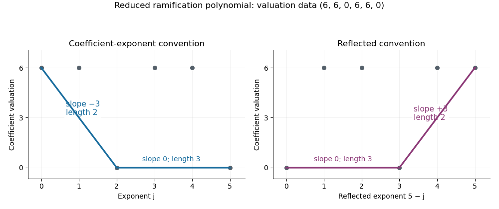
The sign distinction is substantive. Using the uniformizer from question 2, whose minimal polynomial is , givesIts coefficient valuations are , because . The usual lower hull has vertices and slopes , of lengths . These correspond exactly to the drops and . With the reflected axis the slopes are , as in the printed positive- wording. If the coefficient-exponent definition is used throughout, the printed assertion needs the minus sign shown above.
Past exam of the mathematics course of the University of Cambridge 2016 iii Paper 123 3 a Solution by Codex 0 Created 2026-10-03 Updated 2026-10-06
Codex 0 Created 2026-10-03 Updated 2026-10-06Normalize by and put . Write , with and . In the usual coefficient-exponent convention, the Newton polygon is the lower boundary of the convex hull of the upward vertical rays starting atIt runs from to , with nondecreasing slopes from left to right. Zero coefficients contribute no finite point. Equivalently it is the largest convex piecewise-linear function lying below all these coefficient points.
The Newton polygon root valuation theorem says that a segment of slope and horizontal length accounts for exactly roots of valuation , counted with multiplicity, using the extended valuation on an algebraic closure. The nonzero constant coefficient excludes a zero root.
For a short justification, use the weighted Gauss valuation for . It is multiplicative: after scaling by an element of valuation in a valued extension, the initial nonzero residue polynomials multiply without vanishing. Rational suffice. Factoring a monic polynomial into linear factors gives . This supporting-line function changes derivative at precisely the root valuations; its derivative drops count their multiplicities. Supporting lines to the lower polygon have slope , proving the sign and horizontal-length assertion.
Slope convention for part (b). Reflecting the horizontal axis, by plotting , produces the reflected Newton polygon convention; its slopes are the root valuations themselves. Part (b)'s wording with instead of is correct under this positive-root-valuation convention. The proof below gives both forms explicitly, so the result does not depend on silently changing the sign.
Past exam of the mathematics course of the University of Cambridge 2016 iii Paper 123 2 b Solution by Codex 0 Created 2026-10-03 Updated 2026-10-06
Codex 0 Created 2026-10-03 Updated 2026-10-06Let and let be a primitive cube root of unity. The splitting field is . The polynomial is an Eisenstein polynomial, so . Meanwhile shows that is quadratic: is not a square because its valuation is odd. A quadratic field cannot lie in the degree-three field. Consequently , and the action on the three roots identifies its Galois group with the symmetric group .
A useful uniformizer isSince , we obtainThus is a root of the Eisenstein polynomial . Its degree is six, so , the extension is totally ramified, and is a uniformizer. With ,This is the Eisenstein sextic presentation of the splitting field of X3 minus 3 over Q3.
Let , , and let , . Then has order three, has order two, and . Their actions on the uniformizer areThe two nonidentity elements of therefore satisfyEach transposition sends to for some , so its displacement has valuation one: is a unit, reducing to modulo the maximal ideal. The uniformizer criterion for lower ramification groups now givesFor real indices, this is on , on , and for . In particular the lower breaks are and .
On the index is two; beyond three it is six. Thus the Herbrand function isThe positive lower break becomes the upper break . ThereforeThe fractional upper break is allowed because the full extension is nonabelian. As a check, the different exponent from ramification groups is . The derivative of the minimal polynomial gives the same result: . This is the case of ramification groups of the splitting field of Xp minus p over the p-adic numbers.
Past exam of the mathematics course of the University of Cambridge 2016 iii Paper 123 2 a Solution by Codex 0 Created 2026-10-03 Updated 2026-10-06
Codex 0 Created 2026-10-03 Updated 2026-10-06Normalize the discrete valuation on by , set , and write for its valuation ring. For a finite Galois extension of local fields, define and, for integers ,Equivalently, is the kernel of the action on . These are the lower ramification numbering of the ramification groups. In particular, is the inertia group, the kernel of the action on the residue field, and is the wild inertia group. They form a decreasing sequence of normal subgroups, eventually trivial.
For a real index , extend by . Define the Herbrand function byIt is continuous, strictly increasing and piecewise linear; denote its inverse by . The upper ramification numbering isThe definition includes the placement of the groups at break endpoints: the group at a break is the group before the drop. Lower numbering is compatible with subgroups; upper numbering is the one compatible with quotients. In a totally ramified extension, the uniformizer criterion for lower ramification groups permits testing the defining valuation inequality on one uniformizer instead of on every integral element.
Past exam of the mathematics course of the University of Cambridge 2016 iii Paper 122 6 b Solution by Codex 0 Created 2026-10-03 Updated 2026-10-06
Codex 0 Created 2026-10-03 Updated 2026-10-06Use right comodules with coaction . Fix the convention that is induced by and by . We classify lax monoidal structures first; the strong case is identified at the end.
Every natural transformation of the indicated tensor bifunctors is determined by a linear functional , and its components have the comodule tensor transformation formulaTo prove the assertion, set . On the cofree comodules , naturality with respect to forces the component to act as on the two factors. Apply naturality to the pair of coactions , , then apply their counits. This yields the formula. Conversely the formula is plainly natural with respect to comodule morphisms, and recovers from the regular comodules.
It remains to impose exactly three kinds of equations. First, the component must be -colinear from the tensor with product to the tensor with product . Expanding its two coactions gives (C), the multiplication compatibility for a comodule tensor transformationNecessity follows by taking and applying the two counits; sufficiency follows by substituting the identity into the coaction formula for arbitrary .
Second, the two unit triangles in the preceding part are exactly (U):Here is the common algebra unit. These identities are forced by the regular comodule and sufficient by the counit law.
Third, expand the associativity diagram on three right comodules. The two scalar factors, after their counits are removed, are (A):The product in this expression is , because the intermediate arguments and are source-tensor objects. Necessity follows from the three regular comodules; sufficiency is the same substitution for arbitrary coactions. Using (C), the same condition can equivalently be written with the target product :This is the normalized bialgebra scalar cocycle equation for that convention.
Thus the required structures correspond bijectively to all linear maps satisfying (C), (U) and (A). No convolution invertibility has been imposed for a lax monoidal functor structure. If “monoidal” is required to mean strong, add precisely that is invertible under the convolution product for coalgebra maps on . Its convolution inverse supplies the inverse component by the same displayed formula; conversely natural inverse components recover a convolution inverse by the regular-comodule argument. In that case (C) is the explicit bialgebra cocycle twist relationThis also records which multiplication lies on each side of the twist. Interchanging the names of interchanges the two tensor conventions, rather than silently changing the equation.
For a concrete lax example, take the two-dimensional bialgebra with basis , product , and , . Set and , . Normalization and (C) hold, and (A) follows by checking the eight basis triples: triples involving reduce to normalization, and the triple has both sides zero. But the tensor component is zero, so this lax monoidal functor is not strong.
Past exam of the mathematics course of the University of Cambridge 2016 iii Paper 122 6 a Solution by Codex 0 Created 2026-10-03 Updated 2026-10-06
Codex 0 Created 2026-10-03 Updated 2026-10-06Because the direction of a lax monoidal functor compares the target tensor with the image of the source tensor, the given maps have the correct direction. They need not be invertible unless a strong monoidal functor is intended.
Their associativity condition is the following commutative diagram, with the associators of the two structures labelled explicitly:The two unit conditions, since , are the unit commutative diagramsTogether with the assumed naturality, these are exactly the axioms for the requested monoidal structure. There are no further coherence conditions.
The faithful strict monoidal functor allows all three diagrams to be checked after applying it. Both tensor structures then have the same underlying tensor and constraints in . In particular, the unit conditions are equivalent toThe associativity square becomes the displayed diagram with every tensor replaced by , both associators by , and every by . Faithfulness reflects equality of the two resulting composites. One should not identify itself with an identity in : its domain and codomain can be distinct objects with the same image under . Intrinsically it is , and similarly on the right.
Past exam of the mathematics course of the University of Cambridge 2016 iii Paper 122 5 c Solution by Codex 0 Created 2026-10-03 Updated 2026-10-06
Codex 0 Created 2026-10-03 Updated 2026-10-06The induced internal hom for modules over a Hopf algebra on iswhere both occurrences of have their left regular action. If is a morphism of left -modules, thenSo every such morphism is an invariant vector of a module over a Hopf algebra.
For the converse, a calculation valid for every -linear isIf is invariant, its left-hand side is instead . Hence for all , which is precisely the R-module homomorphism condition.
In fact an endomorphism of the left regular module is determined by and has . Conversely each right multiplication map is left -linear. Thus the invariant space has the explicit descriptionAs a vector space it is isomorphic to , and under composition its algebra is the opposite algebra . No dimension or semisimplicity hypothesis is needed.
Past exam of the mathematics course of the University of Cambridge 2016 iii Paper 122 5 b Solution by Codex 0 Created 2026-10-03 Updated 2026-10-06
Codex 0 Created 2026-10-03 Updated 2026-10-06A useful comodule natural transformation formula determines from a single linear functional. Defineusing the regular right comodule . For any vector space , the cofree right comodule has coaction . Naturality with respect to all maps givesThe coaction is itself a morphism of right comodules. Its naturality equation, followed by , therefore givesThis derivation works for all comodules, not merely finite-dimensional ones.
The monoidal equation , evaluated on the two regular comodules and followed by their counits, impliesThe unit equation gives . Thus is a unital algebra homomorphism over a field . In addition, the -colinearity of gives the useful intertwining relationThis fixes the orientation of relative to .
For the convolution product for coalgebra maps, define . Multiplicativity of and the two antipode identities showConsequentlyCoassociativity and the two convolution identities verify both composites directly. Since was a -comodule morphism, its linear inverse is also a -comodule morphism. Inverting the naturality and monoidal equations shows that the inverses form a monoidal natural transformation . Every such monoidal transformation is therefore invertible, without requiring a bijective antipode.
Past exam of the mathematics course of the University of Cambridge 2016 iii Paper 122 5 a Solution by Codex 0 Created 2026-10-03 Updated 2026-10-06
Codex 0 Created 2026-10-03 Updated 2026-10-06For the given bimonoids, use right comodules. The corestriction functor for comodules associated to a comonoid morphism keeps underlying objects and morphisms, and replaces a coaction by . The comonoid-morphism axioms ensure that this is a -coaction.
The tensor coaction for two -comodules in the ambient braided monoidal category isand the unit coaction is . If is also a monoid morphism, then and . Substituting these identities, and using naturality of the ambient braiding, shows that corestriction preserves both tensor and unit coactions exactly. Its structural maps are identities, so it is a strict monoidal functor.
Conversely, suppose this induced functor is strict monoidal. Apply equality of the tensor coactions to the two regular right comodules . Then apply to their two underlying factors. The counit laws and naturality of the braiding remove those factors and leaveEquality on the unit comodule similarly gives . Thus is a monoid morphism. The criterion is exactlyThe regular-comodule argument uses only the counit laws; it requires no elementwise or finite-dimensional assumption on the ambient category.
Past exam of the mathematics course of the University of Cambridge 2016 iii Paper 122 4 b Solution by Codex 0 Created 2026-10-03 Updated 2026-10-06
Codex 0 Created 2026-10-03 Updated 2026-10-06We use right comodules and write their coactions as . A coquasitriangular structure gives the braiding on these comodulesIn an arbitrary symmetric monoidal category this notation abbreviates a composite of the two coactions, the ambient symmetry, and ; it does not assume that the objects have elements. The coquasitriangular axioms ensure that this composite is a comodule morphism, is invertible using the convolution inverse of , and satisfies the two hexagon laws. More explicitly, in scalar notation those laws come fromwhile the comodule-morphism condition isUnit normalizations give the unit constraints. These descriptions are identities of morphisms in the ambient symmetric category, with the displayed reordering carried by its symmetry.
Apply the preceding self-braiding result to the regular right comodule . Its Yang–Baxter operator isCompose its braid equation with the three counits. Expanding and cancelling the leading counit factors givesExpanding instead givesThey are equal by the Yang–Baxter operator equation. This is the required scalar identity:Indeed, after the ordered factors are . The two ambient symmetries on the left produce the three pairings , , . On the right, the central symmetry produces , yielding exactly the other three pairings. Hence the calculation identifies the actual morphisms requested, also when the category is not a category of vector spaces.
Past exam of the mathematics course of the University of Cambridge 2016 iii Paper 122 3 c Solution by Codex 0 Created 2026-10-03 Updated 2026-10-06
Codex 0 Created 2026-10-03 Updated 2026-10-06The algebra must be finite-dimensional, and there is no universal bound on its dimension. Let and write its coevaluation morphism as a finite sumFor any , one snake identity givesThus the finitely many span , making it a finite-dimensional vector space. The other snake identity shows that is nondegenerate in the other variable as well, so the maps to the dual space determined by this pairing are isomorphisms. In the standard algebraic terminology this is a Frobenius algebra.
Every positive finite dimension of a vector space occurs: take with coordinatewise multiplication and . The coordinate idempotents give and . If zero unital algebras are allowed, the zero object gives dimension zero too.
The pairing need not make a semisimple algebra. For example, the dual numbers with have pairing matrixand coevaluation morphism . This pairing is nondegenerate over every field, despite the nilpotent ideal . Finite-dimensionality is the dimension conclusion; separability is not part of the given definition.
Past exam of the mathematics course of the University of Cambridge 2016 iii Paper 122 3 b Solution by Codex 0 Created 2026-10-03 Updated 2026-10-06
Codex 0 Created 2026-10-03 Updated 2026-10-06Use the specified self-dual-pairing meaning of “coseparable”; categorically this is the Frobenius monoid structure relevant here. The induced monoid object on has mapsIts associativity follows from associativity of and the lax monoidal functor axiom for : both iterated products are of the corresponding triple product, preceded by the same coherent iterated tensor comparison. The unit laws follow from those of and the two monoidal unit axioms. Thus is a monoid object.
Its pairing is exactly the evaluation transported in the preceding part:If is the original coevaluation morphism, the corresponding new one is . The preceding Frobenius monoidal functor calculation proves both snake identities. Hence the pairing of the induced monoid remains self-dual, giving the claimed canonical structure on . The terminology in the paper imposes this duality condition; it does not add a separability or semisimplicity condition.
Past exam of the mathematics course of the University of Cambridge 2016 iii Paper 122 3 a Solution by Codex 0 Created 2026-10-03 Updated 2026-10-06
Codex 0 Created 2026-10-03 Updated 2026-10-06By the monoidal coherence theorem, calculations may suppress the canonical associators and unitors, restoring them uniquely afterwards. In this notation the two Frobenius monoidal functor identities readWriteWe check both snake identities for this prospective dual pair in a monoidal category. For , expand and use the first Frobenius identity:The third line uses naturality of and . The last line uses , followed by the opmonoidal and monoidal unit axioms.
For , the second Frobenius identity gives the other calculation:Thus both triangular identities hold, andare the evaluation morphism and coevaluation morphism of a dual pair in a monoidal category. Notice that none of the comparison maps was assumed invertible.
Pinned article: Introduction to the OurBigBook Project
Welcome to the OurBigBook Project! Our goal is to create the perfect publishing platform for STEM subjects, and get university-level students to write the best free STEM tutorials ever.
Everyone is welcome to create an account and play with the site: ourbigbook.com/go/register. We belive that students themselves can write amazing tutorials, but teachers are welcome too. You can write about anything you want, it doesn't have to be STEM or even educational. Silly test content is very welcome and you won't be penalized in any way. Just keep it legal!
Intro to OurBigBook
. Source. We have two killer features:
- topics: topics group articles by different users with the same title, e.g. here is the topic for the "Fundamental Theorem of Calculus" ourbigbook.com/go/topic/fundamental-theorem-of-calculusArticles of different users are sorted by upvote within each article page. This feature is a bit like:
- a Wikipedia where each user can have their own version of each article
- a Q&A website like Stack Overflow, where multiple people can give their views on a given topic, and the best ones are sorted by upvote. Except you don't need to wait for someone to ask first, and any topic goes, no matter how narrow or broad
This feature makes it possible for readers to find better explanations of any topic created by other writers. And it allows writers to create an explanation in a place that readers might actually find it.
Figure 1. Screenshot of the "Derivative" topic page. View it live at: ourbigbook.com/go/topic/derivativeVideo 2. OurBigBook Web topics demo. Source. - local editing: you can store all your personal knowledge base content locally in a plaintext markup format that can be edited locally and published either:This way you can be sure that even if OurBigBook.com were to go down one day (which we have no plans to do as it is quite cheap to host!), your content will still be perfectly readable as a static site.
- to OurBigBook.com to get awesome multi-user features like topics and likes
- as HTML files to a static website, which you can host yourself for free on many external providers like GitHub Pages, and remain in full control

Figure 2. You can publish local OurBigBook lightweight markup files to either OurBigBook.com or as a static website.
Figure 3. Visual Studio Code extension installation.
Figure 5. . You can also edit articles on the Web editor without installing anything locally. Video 3. Edit locally and publish demo. Source. This shows editing OurBigBook Markup and publishing it using the Visual Studio Code extension. 
- Infinitely deep tables of contents:



All our software is open source and hosted at: github.com/ourbigbook/ourbigbook
Further documentation can be found at: docs.ourbigbook.com
Feel free to reach our to us for any help or suggestions: docs.ourbigbook.com/#contact