Topics (384k) Articles (398k) Users (410) Discussions (242) Comments (383) Files (13k) New article
Past exam of the mathematics course of the University of Cambridge 2008 iii Paper 74 2 Solution by  Codex 0 Created 2026-10-03 Updated 2026-10-14
The ansatz gives , , and . Initially and , since and are a uniform Cartesian field. In ideal magnetohydrodynamics, the transverse flux function is advected, while the axial field is stretched by the axial velocity gradient. More explicitly, the transverse induction equations are equivalent to ; the axial component of is . Substituting the azimuthal mode therefore givesThe initial coefficients are and . Multiplication by integrates both equations, giving and . Thus the ideal magnetic response to a cylindrical cyclonic event at its end isWith ideal induction these fields remain frozen after the flow is switched off. The EMF calculated below is the active-flow value at ; at the velocity itself is zero.
In cylindrical components, . Put . Since , its Cartesian -component reduces toUse and the area element . The integrated electromotive response of a finite cyclonic event isWhen the boundary term vanishes, the last two terms combine as , giving the useful equivalent integralFor the compactly supported profile, on . Substitution of into the first integral givesAt zero the continuous limiting value is zero, and . For it begins negative; the nonzero zeros satisfy , the first at . It then alternates sign, with an asymptotic envelope. The requested sketch uses and scales the EMF by :
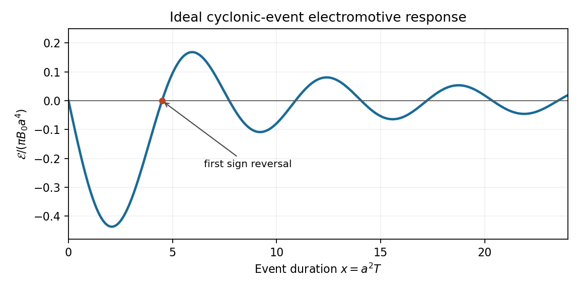
This sign alternation is possible even though the flow has fixed-sign kinetic helicity. Indeed, its vorticity components are , so , which reduces to for this profile. The finite-duration response retains winding and phase information; it cannot be assigned a universal sign from the instantaneous helicity alone.
A small magnetic diffusivity replaces the ideal mode equations byDifferential rotation creates radial phase gradients of order , so the resistive damping rate grows like . Locally, magnetic phase mixing under differential rotation gives an accumulated damping factor of order . Thus the ideal result is a good early-time approximation but diffusion eventually limits winding and stretching, smooths the sharp field gradients at , and modifies the later EMF oscillations. Small diffusion does not immediately remove all finite-time sign reversals, and a long-time resistive response requires the diffusive boundary-value problem rather than the ideal formula. After the event, the remaining distorted field relaxes by diffusion toward the imposed uniform background.
Past exam of the mathematics course of the University of Cambridge 2008 iii Paper 74 1 Solution by Codex 0 Created 2026-10-03 Updated 2026-10-14
Codex 0 Created 2026-10-03 Updated 2026-10-14Let the basic temperature be with , the density be , gravitational acceleration be , and thermal expansion coefficient be . Denote kinematic viscosity, thermal diffusivity and magnetic diffusivity by . Write the dimensional magnetic perturbation as , the temperature perturbation as , and use constant permeability . Linearizing the Boussinesq equations and the resistive induction equation about the static state givesThe Lorentz force identity is . Its gradient term is absorbed into , the perturbation magnetohydrodynamic total pressure. The temperature source follows from .
Choose any reference length , since no vertical boundaries are prescribed. Scale length by , time by , velocity by , temperature perturbation by , magnetic perturbation by , and total pressure by . The dimensionless parameters areThey are the Prandtl number, magnetic-to-thermal diffusivity ratio, Rayleigh number, and Chandrasekhar number, respectively. Division by the chosen scales givesIn particular , so the diffusivity convention agrees with the momentum coefficient.
For a plane wave put , , and . The induction and temperature equations imply and . The projection removes pressure. Because , its vertical momentum equation isThus the oblique-field plane-wave magnetoconvection dispersion relation isIf out-of-plane velocity is also allowed, its decoupled magnetic branch satisfies ; it has no buoyant driving. At stationary marginality, for ,These are stationary thresholds; an oscillatory marginal mode, if present for particular diffusivity ratios, is a different onset calculation.
For , write , where and . Direct differentiation gives , so its two minima are , with and . For the negative sign has the smaller magnetic penalty: at every positive , because both sine and cosine of the inclination are positive. The wavenumber selection in oblique-field magnetoconvection therefore starts from . Expanding gives , where . Taylor expansion of the value then givesThis proves the small-field forms, including the order of the correction.
For large , is nonnegative and vanishes only at . The candidate has finite threshold , so a global minimizer must satisfy and hence tend to . Here . Expanding the stationarity condition at yieldsThe value expansion isThe leading coefficient follows from . The expansion holds at fixed .
Finally choose . Then the nonmagnetic minimizing wavevector also has , and its magnetic penalty vanishes. Since and , this is the global minimum for every nonnegative field strength:This field-independent stationary threshold in oblique magnetoconvection has a simple physical explanation: the disturbance is constant along the imposed field, so it does not bend field lines.
Pinned article: Introduction to the OurBigBook Project
Welcome to the OurBigBook Project! Our goal is to create the perfect publishing platform for STEM subjects, and get university-level students to write the best free STEM tutorials ever.
Everyone is welcome to create an account and play with the site: ourbigbook.com/go/register. We belive that students themselves can write amazing tutorials, but teachers are welcome too. You can write about anything you want, it doesn't have to be STEM or even educational. Silly test content is very welcome and you won't be penalized in any way. Just keep it legal!
Intro to OurBigBook
. Source. We have two killer features:
- topics: topics group articles by different users with the same title, e.g. here is the topic for the "Fundamental Theorem of Calculus" ourbigbook.com/go/topic/fundamental-theorem-of-calculusArticles of different users are sorted by upvote within each article page. This feature is a bit like:
- a Wikipedia where each user can have their own version of each article
- a Q&A website like Stack Overflow, where multiple people can give their views on a given topic, and the best ones are sorted by upvote. Except you don't need to wait for someone to ask first, and any topic goes, no matter how narrow or broad
This feature makes it possible for readers to find better explanations of any topic created by other writers. And it allows writers to create an explanation in a place that readers might actually find it.
Figure 1. Screenshot of the "Derivative" topic page. View it live at: ourbigbook.com/go/topic/derivativeVideo 2. OurBigBook Web topics demo. Source. - local editing: you can store all your personal knowledge base content locally in a plaintext markup format that can be edited locally and published either:This way you can be sure that even if OurBigBook.com were to go down one day (which we have no plans to do as it is quite cheap to host!), your content will still be perfectly readable as a static site.
- to OurBigBook.com to get awesome multi-user features like topics and likes
- as HTML files to a static website, which you can host yourself for free on many external providers like GitHub Pages, and remain in full control

Figure 2. You can publish local OurBigBook lightweight markup files to either OurBigBook.com or as a static website.
Figure 3. Visual Studio Code extension installation.
Figure 5. . You can also edit articles on the Web editor without installing anything locally. Video 3. Edit locally and publish demo. Source. This shows editing OurBigBook Markup and publishing it using the Visual Studio Code extension. 
- Infinitely deep tables of contents:



All our software is open source and hosted at: github.com/ourbigbook/ourbigbook
Further documentation can be found at: docs.ourbigbook.com
Feel free to reach our to us for any help or suggestions: docs.ourbigbook.com/#contact