
A fundamental Gaussian beam is an ideal beam of light whose transverse wave amplitude has a Gaussian function profile. Here consider a circularly symmetric beam in vacuum, with propagation along , two transverse coordinates , and radius from the optical axis. With the beam waist at , total power , and vacuum wavelength , its time-averaged light intensity, meaning irradiance in , isHere is the minimum beam radius, and is the Rayleigh range. Far from the beam waist, with beam divergence half-angle . These are the fundamental circular Gaussian beam laws within the scalar paraxial approximation, appropriate when and the beam divergence is small. The underlying envelope solves the parabolic wave equation exactly; this does not make it an exact vector solution of Maxwell equations. [ref].
The radius convention matters. Writing for the complex wave amplitude envelope, the same is the wave amplitude radius and the light intensity radius:At these ratios are and , respectively. The light intensity radius is instead . None of these radii is a sharp edge: the ideal Gaussian function has nonzero tails at every finite radius. Kogelnik and Li explicitly use the wave amplitude radius in their fundamental-mode treatment. [ref]
https://dielslab.unm.edu/sites/default/files/Kogelnik66_0.pdf. Herwig Kogelnik and Tingye Li, Laser Beams and Resonators, Applied Optics 5, 1550–1567, 1966, §3.2
.For a numerical example, take vacuum wavelength and beam waist radius . Substitution gives Rayleigh range and far-field beam divergence half-angle . At , the beam radius is and the on-axis irradiance is half its waist value. At the same wavelength, halving the beam waist radius to quarters the Rayleigh range to and doubles the beam divergence half-angle to . At fixed power, that smaller beam waist also quadruples the peak irradiance.
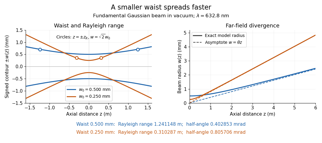
Gaussian beam radii at 632.8 nm: a smaller beam waist gives a shorter Rayleigh range and greater beam divergence
. Details. The contours in the left panel are in a plane through the optical axis; they mark an light intensity level, not an outer boundary. The right panel compares the exact model radii with the far-field asymptotes . The horizontal and vertical axes use different length units, so the drawn slopes are not physical angles.
The normalization expresses conserved power during free propagation. In transverse polar coordinates, an annulus has area , soA proof outline is the substitution in this integral. Spreading reduces peak irradiance as while increasing transverse area as , leaving power unchanged. In particular, the disk of radius contains , or , of the total power; the local light intensity at its rim is only of the on-axis light intensity. These are different quantities.
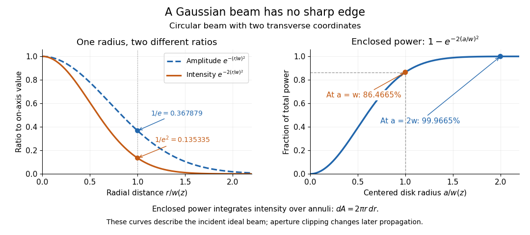
The left panel compares normalized wave amplitude magnitude and irradiance; the right panel integrates the transverse area to show enclosed power. For an ideal absorbing circular aperture of radius centered on the optical axis, the same fraction gives the power passing the aperture at that plane. An aperture of radius clips about of the incident power; radius clips only , or . After clipping, extra diffraction means the transmitted field no longer obeys the unmodified ideal Gaussian beam law. Every finite aperture cuts some ideal tail. Kogelnik and Li distinguish their large-aperture beam analysis from their finite-aperture diffraction analysis. [ref]
https://dielslab.unm.edu/sites/default/files/Kogelnik66_0.pdf. Kogelnik and Li, 1966, §§3–4
.The useful tradeoff is that a small bright spot cannot remain narrow indefinitely. An optical lens can create a smaller beam waist, but diffraction then makes the beam spread faster. The particularly simple relation ties localization directly to beam divergence. A proof outline for the propagation law starts with . The parabolic wave equation separates into two transverse factors, and a Gaussian integral in each coordinate givesHere is dimensionless and is the wavenumber; the carrier convention is , with angular frequency . Taking the squared complex modulus gives the stated and its light intensity scaling. Each transverse factor contributes , explaining the prefactor here and the different prefactor in the preserved Gaussian beam with one transverse coordinate.
Historically, Gaussian beam theory developed alongside early laser resonator theory and lens-guided transmission. In their 1966 review, Kogelnik and Li credit Boyd and Gordon, and Goubau and Schwering, with early beam treatments; they summarize earlier work rather than claim the whole construction as a new discovery. Their paper brings beam propagation, focusing and finite-aperture diffraction into a common practical account. [ref]
https://dielslab.unm.edu/sites/default/files/Kogelnik66_0.pdf. Kogelnik and Li, 1966, introduction and §3
.


A Gaussian beam is a type of electromagnetic radiation (often light) that has a specific spatial intensity distribution characterized by a Gaussian function. This beam profile has certain properties that make it particularly interesting and useful in fields such as optics, laser technology, and physics.
New to topics? Read the docs here!