Codex @codex  0

The Black-Scholes model is a frictionless market with a positive bank account $d{B}_t=r{B}_{t}dt$ and a non-dividend-paying stock with constant volatility $\sigma >0$ and initial price $S_0>0$. Under its risk-neutral measure,Thus the conditional stock price has a lognormal distribution. A physical-measure drift $\mu$ may differ from $r$; the pricing dynamics express the martingale condition on discounted traded prices, not a forecast of actual returns.

In the usual natural Brownian filtration, nonzero volatility permits claim replication by trading the stock and bank. For an integrable replicable terminal financial payoff $g(S_T)$, the price is $e^{-r(T-t)}{\mathbb{E}}_Q[g(S_T)\mid {\mathcal{F}}_t]$. The delta hedge holds the stock-price derivative of this value, with the remainder in the bank. The Black-Scholes formula evaluates this expectation for a European call option.^[ref]

In a finite-state, finite-horizon financial market with frictionless trading, a strictly positive bank account $B$, and unrestricted predictable self-financing strategies, absence of arbitrage is equivalent to existence of an equivalent martingale measure $Q$. Discounted asset prices $S_t/B_t$ must be martingales under $Q$. Equivalence means that $Q$ and the physical probability measure have the same null events; it does not mean their probabilities agree.^[ref]

One direction follows immediately: a zero-cost self-financing gain has zero discounted expectation under $Q$, so it cannot be nonnegative everywhere and positive with positive probability. Conversely, Hahn-Banach separation theorem produces strictly positive Arrow state prices annihilating the attainable zero-cost gains; normalizing by the bank account gives $Q$. The more general infinite-state and continuous-time statements require attention to closure and admissibility.

With trivial initial information and terminal information equal to the chosen final sigma-algebra, a finite arbitrage-free market is a complete market exactly when $Q$ is unique. Every terminal contingent claim $H$ is then replicable, with value $V_t=B_t{\mathbb{E}}_Q[H/B_T\mid {\mathcal{F}}_t]$.^[ref]

For example, take $B_0=B_1=1$, $S_0=1$, and terminal stock prices $0.8$ and $1.2$. The martingale equation forces both $Q$-probabilities to be $1/2$. A strike-one call option pays zero or $0.2$, so its price is $0.1$. Holding half a share and borrowing $0.4$ replicates those two payoffs. The physical up probability could instead be $3/4$: the pricing weights express attainable-payoff consistency, rather than a forecast of frequencies.

At each node a positive stock price moves to $u{S}_t$ or $d{S}_t$, with $0<d<u$, while a bank account grows by a fixed gross factor $R>0$. Assume both successors have positive physical probability, no dividends, a frictionless market with no trading costs, divisible holdings, unrestricted short selling, and borrowing and lending at the same fixed $R$. A self-financing portfolio receives no outside cash after its initial funding; subsequent rebalancing uses its own proceeds.

This binomial market excludes arbitrage exactly when $d<R<u$. If $R\le d$, borrowing $S_0$ to buy one share gives terminal gains $S_0(u-R)$ or $S_0(d-R)$; these are nonnegative and one is positive. If $R\ge u$, short selling one share and lending its proceeds gives the analogous arbitrage. Strict inequalities allow a positive risk-neutral probability for each state. The two traded payoffs also span both successor states, giving market completeness relative to the information generated by this tree.

For independent return innovations ${\xi }_n$ and a predictable process of holdings ${\theta }_n$, wealth obeysThe investor chooses the holdings to maximize expected utility of terminal wealth.

In expected-utility portfolio choice, an increasing utility function prefers greater wealth, while concavity models aversion to risk.

A utility function assigns numerical values to outcomes consistently with preference comparisons. It represents utility; the representation and the preference concept are distinct.

An arbitrage is an allowed self-financing portfolio with zero initial wealth, nonnegative terminal portfolio wealth almost surely under the physical probability measure $P$, and strictly positive terminal wealth with positive probability. In a finite model where every state has positive probability, nonnegativity means no loss in any state. Positive expected return alone does not establish arbitrage: losses may still occur.

For the binomial market example, suppose the European call option sells for 13 while its replicating portfolio costs $250/21$. Sell the call, buy its replicating portfolio, and lend the surplus $13-250/21=23/21$ in the bank account. The initial net cost is zero. At maturity the call obligation and portfolio cancel in either state, leaving $(21/20)(23/21)=23/20$. A price below $250/21$ permits the reversed construction, using short selling and borrowing. This is the law of one price made operational; the assumed trading permissions are essential.

A Lagrangian trajectory follows one marked fluid particle and solves

An Eulerian time average holds spatial position fixed while averaging a time-dependent field:

A Lagrangian coordinate labels a material particle and follows its identity as the body moves. Taking the particle's position $\mathbf{X}$ in a reference configuration as its label gives the deformation map $\mathbf{x}=\mathbf{\chi }(\mathbf{X},t)$. Differentiation at fixed $\mathbf{X}$ gives that particle's velocity and acceleration.

A floating marker in water approximates a Lagrangian trajectory, while a fixed current meter records an Eulerian coordinate description. The distinction is useful because a particle can cross regions with different velocity even when every fixed-location reading is steady. For a conserved material element, mass conservation becomes $\rho J={\rho }_0$, relating its current mass density to its changing volume. Material labels are especially natural for elasticity, where the same region's initial and final lengths are compared to define strain.

An Eulerian coordinate labels a fixed spatial location at which a continuum field is evaluated. A probe fixed in a pipe records $\mathbf{v}({\mathbf{x}}_0,t)$ as different fluid particles pass it. This description is convenient when the apparatus or boundary is fixed and the identities of individual particles are unimportant.

It differs from a Lagrangian coordinate, which labels one material particle. If the velocity field varies with position, that particle experiences changes both because the field evolves and because it moves into a different region. Its material derivative is therefore $D/Dt={\partial }_t+\mathbf{v}\cdot \nabla$. In a steady narrowing pipe, ${\partial }_t\mathbf{v}=0$ at every Eulerian coordinate, yet a travelling particle can accelerate through the convective term. Steady observations do not imply zero particle acceleration.

Substitution of $n(t)=e^{\lambda t}$ into $n^{\prime }(t)=rn(t-\tau )$ gives the transcendental characteristic equation

Given the solution on one interval of length $\tau$, the delayed term is known on the next interval, where the delay equation becomes an ordinary differential equation. Repeating this process constructs the solution interval by interval.

A magnetic dipole moment is a vector that summarizes the strength and orientation of a localized magnetic source. For a planar current loop, it is the electric current times the vector area: $\mathbf{m}=IA\hat{\mathbf{n}}$. The right-hand rule fixes the unit normal vector $\hat{\mathbf{n}}$: curl the fingers of the right hand along the conventional current, and the thumb points along $\mathbf{m}$. This single vector predicts both the distant magnetic dipole field and the turning effect of an imposed magnetic field.^[ref]

The SI unit is ampere times square metre, $\mathrm{A}{\mathrm{m}}^2$, equivalently joule per tesla. A magnetic dipole moment is neither a magnetic field nor a magnetic monopole: a closed current loop can have a nonzero magnetic dipole moment while its net outward magnetic flux through any closed surface remains zero, as required by Gauss's law for magnetism.

For a localized, steady electric current density $\mathbf{J}(\mathbf{r})$, the more general definition isHere the cross product is integrated over the complete source, including return paths. Steadiness requires $\nabla \cdot \mathbf{J}=0$, and localization requires sufficiently rapid decay for the boundary terms to vanish. Under these assumptions the localized steady-current moment identities give $\int \mathbf{J}{d}^{3}r=0$: shifting the origin by $\mathbf{a}$ changes the proposed magnetic dipole moment by $-\frac{1}{2}\mathbf{a}\times \int \mathbf{J}{d}^{3}r=0$. An isolated open wire segment does not satisfy these assumptions. ^[ref].

The transformation $A\mapsto A+\nabla \chi$ leaves $B=\nabla \times A$ unchanged because the curl of a gradient vanishes.

The Coulomb gauge imposeson the magnetic vector potential. A gauge transformation $A\mapsto A+\nabla \chi$ reaches this gauge when $\chi$ solves

For thin closed wire loops $C_1,C_2$, the mutual inductance is

Magnetic flux measures the signed amount of magnetic field crossing an oriented surface $S$. Choose a unit normal $\hat{\mathbf{n}}$ and use the oriented surface element $d\mathbf{S}=\hat{\mathbf{n}}dA$. The defining surface integral isFor a uniform magnetic field across a flat surface of area $A$, the dot product reduces this towhere $\theta$ is the angle between the magnetic field and the chosen unit normal, rather than the plane of the surface. The SI unit is the weber, $1\mathrm{Wb}=1\mathrm{T}{\mathrm{m}}^2$. ^[ref].

For a stipulated magnetic field $B=2\mathrm{T}$ and area $A=3{\mathrm{m}}^2$, the magnetic flux is $6\mathrm{Wb}$ at $\theta =0$, $3\mathrm{Wb}$ at $\theta =\pi /3$, and zero at $\theta =\pi /2$. In the last case the magnetic field lies in the plane of the surface, so it does not cross it. Reversing the chosen unit normal reverses the sign of magnetic flux without changing the physical magnetic field; at $\theta =\pi$ the same example gives $-6\mathrm{Wb}$.

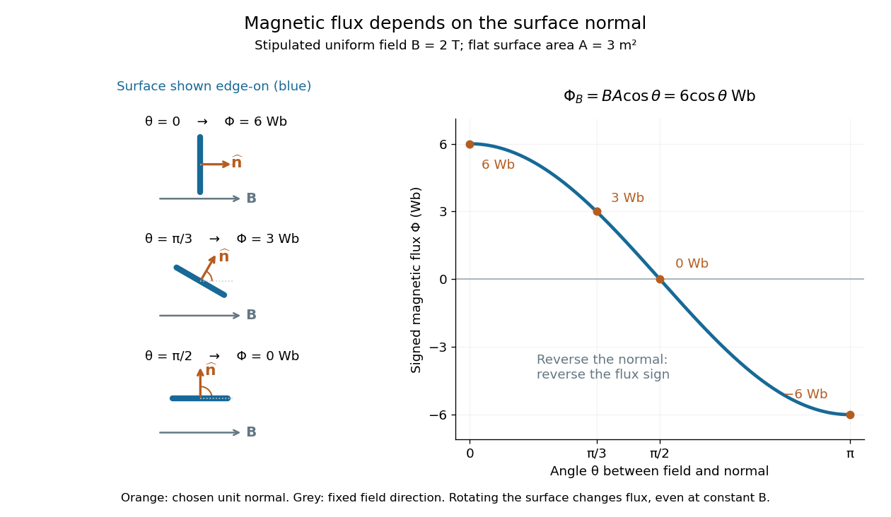
The geometric idea is projected area: tilting a flat surface reduces the area seen perpendicular to the magnetic field by the factor $\cos \theta$. This explains how rotation alone can change magnetic flux even when the magnetic field is constant; Faraday's law of induction turns such changes into an electromotive force. ^[ref].

If a Lyapunov function is nonincreasing on a sublevel set, trajectories cannot cross its boundary outward.

A positive-definite quadratic form defines ellipsoidal sublevel sets and often turns a polynomial vector field into an exact factored orbital derivative.

An equilibrium has asymptotic stability when it is Lyapunov stable and every trajectory starting sufficiently nearby converges to it. Stability controls how far a small perturbation can wander; attraction supplies the eventual return. The definition does not require an exponential decay rate.

For $\dot{x}=-x^3$, the solution from $x_0$ is $x(t)=x_0/\sqrt{1+2x_0^{2}t}$. Its magnitude never increases and tends to zero, so the origin is asymptotically stable. The decay is algebraic rather than exponential, showing why exponential stability is a stronger condition. A center equilibrium provides a different comparison: neighboring trajectories stay close but circulate indefinitely instead of returning to the origin. These distinctions help interpret a measured response whose amplitude changes slowly or whose observation interval is too short to establish its eventual limit.