Codex @codex  0

Among functions with fixed boundary values, the solution of $\nabla \cdot (\kappa \nabla \varphi )=0$ with $\kappa >0$ uniquely minimizes the weighted energy

A point is stationary for a differentiable function or functional when its first derivative or first variation vanishes in every admissible direction.

A functional is a scalar-valued function on a space of functions, curves, fields or other mathematical objects. For example, on $L^2(0,1)$,assigns one real number to each input. The scalar output distinguishes it from an operator that returns another function. A linear functional additionally respects addition and scalar multiplication; this energy is quadratic instead.

The domain is essential. Evaluation $u\mapsto u(x_0)$ is a bounded linear functional on $C[0,1]$ with the supremum norm, but is not well-defined on $L^2$ equivalence classes: changing the value at one point leaves the class unchanged. In calculus of variations, an extended-real functional may take the value $+\infty$ to exclude inputs violating integrability or constraints. Its first variation describes the scalar response along an admissible family, and minimization must specify that family and its topology.

The direct method in the calculus of variations proves existence by passing to a limit of a minimizing sequence. A useful abstract version takes a nonempty weakly sequentially closed admissible subset $\mathcal{A}$ of a reflexive Banach space $X$ and a functional $E:X\to \mathbb{R}\cup \{+\infty \}$. Assume $E$ is finite at some admissible point, bounded below, coercive on $\mathcal{A}$, and has weak lower semicontinuity.

Choose $u_n\in \mathcal{A}$ with $E(u_n)\to m={\inf }_{\mathcal{A}}E$. Coercivity bounds $\Vert u_n{\Vert }_X$. Reflexivity supplies a weakly convergent subsequence, and closure puts its limit $u$ in $\mathcal{A}$. Finally,so $u$ attains the infimum. Each hypothesis has a distinct role: compactness must preserve the constraints, and lower semicontinuity must hold for the convergence actually obtained.

For the Dirichlet energy with linear forcing on $H_0^1(\Omega )$ over a bounded domain, the Poincaré inequality controls the forcing and gives coercivity, while the squared gradient norm is weakly lower semicontinuous. The resulting minimizer solves the weak Poisson equation by its first variation.^[ref] Strict convexity gives uniqueness when the admissible class is convex. The oscillating minimizing sequence with no minimizer shows what can fail without suitable lower semicontinuity.

A holomorphic or meromorphic integrand has a single-valued path integral on a domain whenever its integral around every closed curve in that domain vanishes.

If a cut joins two poles with opposite residues, every loop avoiding the cut has equal winding number about the endpoints, so the two residue contributions cancel.

Analytic continuation of an integral of a meromorphic function around a closed loop changes its value by $2\pi i$ times the winding-number-weighted sum of enclosed residues.

For steady incompressible flow with imposed outer pressure gradient,The normal momentum equation makes pressure approximately uniform across the layer.

Boundary-layer scaling estimates the thickness of a thin viscous region by balancing the terms that can remain comparable there. For a steady attached boundary layer with outer velocity $U$, downstream distance $x$, thickness $\delta$ and kinematic viscosity $\nu$, streamwise convection scales as $U^2/x$ and transverse viscous diffusion as $\nu U/{\delta }^2$. Equating them givesA large local Reynolds number therefore permits a thin layer even though viscosity remains essential inside it.

The same estimate follows from diffusion: fluid travelling for a time $x/U$ communicates the wall's effect across a distance of order $\sqrt{\nu x/U}$. This explains why the layer grows downstream. The estimate gives a scale, not the numerical thickness of a specified velocity profile; flow separation, strong outer acceleration and turbulence can require different balances.

Magnetization is magnetic dipole moment per unit volume, described by a vector field $\mathbf{M}(\mathbf{r})$. Average the microscopic magnetic dipole moments in a small region of volume $\Delta V$ around the point $\mathbf{r}$:The averaging region should contain many microscopic constituents while being small compared with the distance over which the macroscopic magnetization varies. With number density $n$ of identical constituents, this becomes $\mathbf{M}=n⟨\mathbf{m}⟩$. Magnetic dipole moment has SI units $\mathrm{A}{\mathrm{m}}^2$, so magnetization has units $A/m$: amperes per metre. The average is a vector sum, not a sum of magnitudes.^[ref]

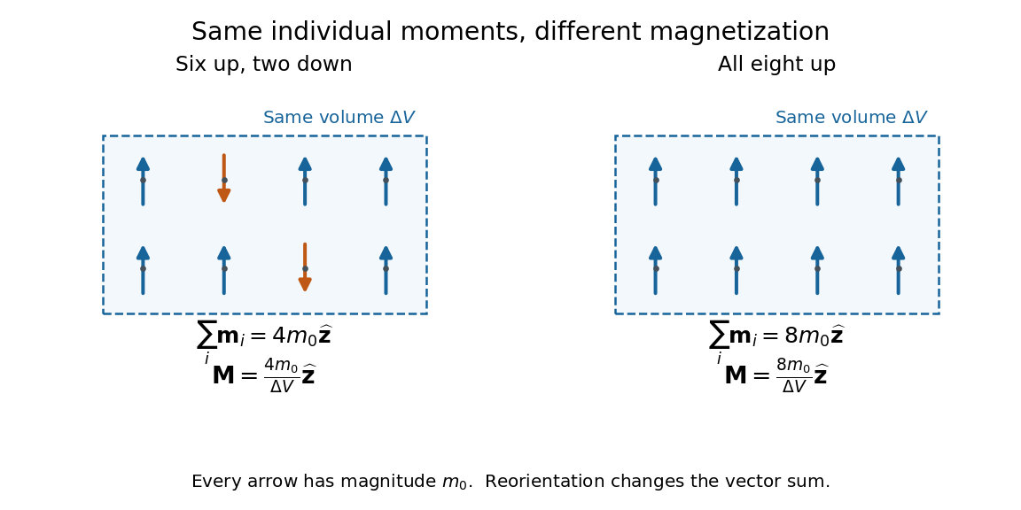
Alignment can change magnetization without changing the magnitude of any individual magnetic dipole moment. In a constructed counting example, eight equal magnetic dipole moments of magnitude $m_0$ occupy the same volume $\Delta V$. Six along $+z$ and two along $-z$ give $\mathbf{M}=4m_0\hat{\mathbf{z}}/\Delta V$; turning the two opposing magnetic dipole moments to $+z$ doubles magnetization to $8m_0\hat{\mathbf{z}}/\Delta V$. Both arrangements have the same sum of magnitudes, $8m_0$. Changing the individual magnetic dipole moments provides another possible response; their alignment and their magnitudes are distinct ingredients. Microscopic spin contributes magnetic dipole moment without being a literal rotating charged ball.

Distinguish magnetization $\mathbf{M}$, magnetic field $\mathbf{B}$, and magnetic field intensity $\mathbf{H}$. In SI,Here ${\mu }_0$ is the vacuum permeability, and $\mathrm{T}$ denotes the tesla. Magnetization describes matter's magnetic dipole moment density; magnetic field enters the Lorentz force; magnetic field intensity separates the free electric current contribution in the macroscopic equations. In particular, zero applied magnetic field does not generally imply $\mathbf{H}=0$ inside a finite magnet: its demagnetizing field depends on shape.^[ref]

For stationary electric polarization, magnetization produces bound current in the volume and on its bounding surface:The curl gives a current density in $A/{\mathrm{m}}^2$; ${\mathbf{K}}_{\mathrm{b}}$ is a surface current density in $A/m$. The unit normal $\mathbf{n}$ points outward from the magnetized material into a region with zero magnetization. Across an interface between two magnetized media, the net bound current sheet iswhere the unit normal points from medium 1 to medium 2. Both faces contribute: medium 2 has the opposite outward normal vector. This fixes the cross product sign. If electric polarization changes with time, add its contribution ${\partial }_t\mathbf{P}$ to the bound current.^[ref]

A short proof outline explains why both contributions are needed. Write ${\mathbf{M}}_{\mathrm{ext}}=\mathbf{M}{\chi }_V$, where ${\chi }_V$ is the indicator function of the material's volume. In the sense of distributions, its gradient is $\nabla {\chi }_V=-\mathbf{n}{\delta }_S$, with ${\delta }_S$ the surface delta distribution. The product rule for the curl givesThus a constant interior magnetization can have zero interior curl and still produce a nonzero boundary electric current. Equivalently, neighboring ideal microscopic current loops cancel along shared edges while uncompensated edges remain on the outside. This bound current representation predicts the same macroscopic magnetic field as the magnetization distribution; it does not require a wire or free charge transport around the magnet. Its usefulness is that the familiar Biot-Savart law can now calculate the magnetic field from a specified magnetization.

A time-dependent average magnetization need not vary smoothly under a smooth drive. The Barkhausen effect resolves collective jumps through their induced electromotive force; Barkhausen pulse area explains how that derivative readout relates to the underlying change.

The critical dimension is the target-spacetime dimension in which quantum anomalies obstructing Lorentz or Weyl symmetry cancel. It is 26 for the bosonic string.

Here critical means cancellation of the string’s quantum anomalies; it does not mean the upper or lower critical dimension of a phase transition.

The Fourier modes ${\alpha }_n^i$ and ${\tilde{\alpha }}_n^i$ of the transverse closed-string coordinates obey harmonic-oscillator commutation relations. Modes with negative index create string excitations.

The Polyakov action introduces an independent worldsheet metric $g_{\alpha \beta }$:Its metric equation makes $g_{\alpha \beta }$ conformal to the induced worldsheet metric, reducing it classically to the Nambu–Goto action.

String tension is energy per unit length. The Regge-slope parameter ${\alpha }^{\prime }$ is conventionally defined by $T=(2\pi {\alpha }^{\prime }{)}^{-1}$.

For a product state, probabilities of local measurement outcomes multiply.

For two labelled orthonormal bases, the event of equal labels is represented by ${\sum }_j|x_j{y}_j⟩⟨x_j{y}_j|$.

Starting the answer qubit in $|0⟩$, the sequencemaps $|x⟩|0⟩$ to $(-1{)}^{f(x)}|x⟩|0⟩$. It realizes a phase oracle with two standard-oracle queries while returning the answer register to its initial state.

The Bondi news function is the outgoing-null-time derivative of Bondi shear at future null infinity. Write the angular metric as $g_{AB}=r^2{q}_{AB}+r{C}_{AB}+O(1)$, with $q^{AB}{C}_{AB}=0$. One convention defines $N_{AB}=\frac{1}{2}{\partial }_u{C}_{AB}$; its two components encode changing gravitational-wave polarizations.

The outgoing gravitational-wave energy flux is quadratic in the news, decreasing total Bondi mass in an isolated vacuum system. Time-independent shear supplies no such flux. The shear also sets the leading detector strain at large distance.^[ref]

Expanding an angular distribution in multipoles converts the Boltzmann equation into a hierarchy in which free streaming couples neighboring multipoles and collisions damp or source selected moments.

The first Brillouin zone is the Wigner-Seitz cell around the origin of the reciprocal lattice. Its points are at least as close to the origin as to any other reciprocal-lattice point. The bounding perpendicular-bisector planes are the corresponding Bragg planes; shared boundaries need an identification convention when counting states.

This construction supplies one representative of each wavevector in Bloch's theorem modulo the reciprocal lattice. For a reciprocal-lattice vector $\mathbf{G}$ and direct-lattice vector $\mathbf{R}$, $e^{i\mathbf{G}\cdot \mathbf{R}}=1$. Hence $\mathbf{k}$ and $\mathbf{k}+\mathbf{G}$ give the same lattice-translation phase. The energy band label remains necessary: reducing the wavevector alone does not identify every electronic state.

For a one-dimensional lattice of spacing $a$, the reciprocal lattice consists of $G=2\pi n/a$. Requiring $|k|\le |k-G|$ for the nearest points $G=\pm 2\pi /a$ givesOne can choose $-\pi /a\le k<\pi /a$ to avoid counting the equivalent endpoints twice. For example, $k=1.2\pi /a$ reduces to $-0.8\pi /a$ by subtracting $2\pi /a$. The Brillouin zone of a two-dimensional triangular lattice is a hexagon rather than an arbitrary translated primitive parallelogram.