
At P critical incidence the transmitted P wave travels along the interface. The common horizontal seismic ray parameter is , givingThe resulting seismic head wave radiates back into the slower upper layer.
The required transmitted P wave angle would satisfyTherefore there is no real transmitted P-ray angle. The incidence exceeds the P critical angle ; the transmitted P contribution is evanescent away from the interface rather than a propagating body ray. Reporting would describe critical incidence, not the stated incidence.
The reflected P wave remains in the upper layer. Conservation of horizontal seismic ray parameter gives , so the reflected P angle is from vertical. This is specular reflection at the horizontal interface.
If a restored channel or fan boundary has accumulated displacement since it formed, a constant fault slip rate gives the geomorphic offset-age relationThe right-hand channel jog is of order one to two of the printed m scale bars, so apparent offsets of order – m give about – ka. These are scale-based order-of-magnitude estimates, not surveyed piercing-point offsets: the amount of deflection along an eroding channel is not automatically equal to the tectonic displacement. For example, a reliably restored m marker would imply ka.
These times lie in the late Pleistocene, when global glacial–interglacial changes could alter vegetation, sediment supply and runoff and thereby promote alluvial fan deposition or abandonment. The wide interval spans different climatic phases, so it does not identify one event or prove a climatic cause. More importantly, a channel cut into a fan usually dates channel establishment or abandonment; the fan sediment can be older. Independent optically stimulated luminescence dating, stratigraphic correlation and several matched offsets are needed to assign a depositional age and test a climatic correlation.
A useful deflected stream is the conspicuous incised drainage in the right-hand part of the image. It approaches the fault corridor from the upper-right, follows a short segment along the trace near , then resumes down the fan toward the lower-left. Mark the two bends and the intervening along-fault reach, rather than labeling the whole channel as a fault.
A candidate beheaded stream is the short downstream gully in the fan immediately to the right of the central wide river, near : its head terminates at or near the cross-cutting fault corridor without an obvious continuation into a substantial upstream catchment. Mark it as a candidate abandoned/cut-off channel, and distinguish it from the active continuous drainage farther right. A displaced upstream counterpart, sediment infill or a field profile would strengthen that identification; optical appearance alone cannot uniquely establish every former channel connection.
Trace the subtle, approximately straight strike-slip fault that cuts across the dissected fan surfaces, descending to the right in the image. In normalized map coordinates measured from the upper left, a tracing corridor runs approximately from through , and toward . The broad central river interrupts the surface expression; extend the trace across that gap cautiously rather than following the river downstream.
The systematic jogs of small channels, particularly the conspicuous right-hand drainage, support right-lateral strike-slip faulting: draw arrows parallel to the trace, with the upper-side block toward the image right/down and the lower-side block toward the image left/up. Restore paired channel segments by reversing that sense and check that the fan rills align better. An isolated channel bend can have an erosional origin, so the consistent set of bends is stronger evidence than any one bend. No cardinal azimuth is asserted because Attachment B provides no north arrow.
A blind reverse fault can shorten and bend its cover into a fault-propagation fold or other growing anticline. At the fold crest, bending can create shallow extension and secondary normal faults or tension fissures, even though the regional deformation is shortening. Bedding-parallel flexural slip, local backthrusts and fold scarps can also break the surface.
Thus a shallow surface break need not be the upward continuation of the main seismogenic thrust fault. The expected association is distributed deformation related to the uplifted fold; its detailed pattern depends on cover layering, fold geometry and shallow strength. The broad frontal relief in Attachment A is compatible with this possibility, but the image alone does not establish a unique earthquake rupture history.
After removing orbital, topographic and atmospheric contributions, an earthquake InSAR radar interferogram would show elongated displacement lobes and generally closed or nested fringes associated with uplift and horizontal shortening of the hanging wall. Each full phase cycle represents of line-of-sight displacement, where is radar wavelength; equivalently , with sign fixed by processing convention.[ref]
Interferometry by NASA. Phase differencing, nuisance contributions and half-wavelength displacement per fringe
If primary slip reaches the surface, expect a displacement discontinuity across the surface trace: fringes can terminate or change abruptly there, and large near-fault gradients or disturbed ground may decorrelate. For a blind reverse fault, the elastic displacement field is continuous at the ground surface and spread over a broader zone, giving smoother gradients and fringes over the uplifted fold. A blind rupture can still create sharp local gradients or secondary faulting.
The exact colour order, number of fringes and sign of the displacement lobes cannot be fixed from this shaded relief alone. They depend on slip, depth and radar look direction; uplift is only one contribution to line-of-sight displacement.
Use normalized image coordinates within the map rectangle, with at its upper left and at its lower right. A principal candidate thrust fault trace follows the sharp, approximately diagonal southwestern edge of the dissected high ground on the right: a practical tracing guide passes nearMark the upland, upper-right side as hanging wall and the smoother, lower-left basin side as footwall for a thrust dipping beneath the uplands. Use broken lines through the gaps, not one asserted continuous exposed rupture. A subsidiary candidate frontal segment follows the basin-facing edge of the isolated dissected ridge on the left, approximately through to ; place teeth toward its locally higher ridge side.
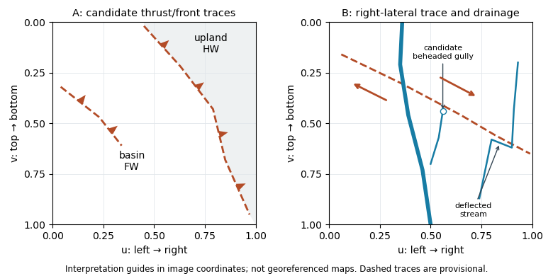
Original interpretation guides for both attachments: provisional traces, block motion and drainage markers in normalized image coordinates
. Details. 
These are geomorphic interpretations of mountain fronts and scarps, not measured subsurface dip directions. On a conventional north-up reading the principal trend is broadly northwest–southeast, but the supplied map has no north arrow: the image-relative coordinates are the reproducible identification. Southwestern illumination means southwest-facing slopes are bright; brightness is a slope-orientation clue, not an elevation contour. Some aligned relief may be a fold scarp or an eroded lithological contact, so field confirmation and topographic profiles would test the candidate traces.
Successive jumps occur at times separated by s. Between and s the plotted function is , periodically extended, with maximum and minimum . Its mean is therefore m, and is an odd function over that centered period.
For the Fourier series convention m and for every ; the nonconstant content consists of sine terms. If denotes the mean directly in the alternative convention , its value is m. Stating the convention resolves the otherwise ambiguous notation.
Regular timing supplies a common interval and a well-defined frequency grid for a standard discrete Fourier transform and Fast Fourier transform. It also makes sample-index lags correspond to fixed physical delays in cross-correlation, autocorrelation and digital filtering. These methods estimate frequency content and characteristic periods, separate instrument or environmental noise from signals, identify arrivals and time delays, and compare ground-motion spectra.
A uniform interval establishes a Nyquist frequency; frequencies above it alias unless filtered before acquisition. Interpolating irregular data onto a regular grid does not undo prior aliasing or fill large gaps with new measurements, and it can alter spectra and create correlated errors. Methods that directly use irregular times are possible, but the ordinary FFT and fixed-lag filter formulas cannot simply treat the original irregular observations as evenly spaced.
Sampling at Hz means s. The target times are therefore , and s, all within the supplied observation range. For bracketing observations, linear interpolation gives . ThusThe estimated displacements are , and . Interpolation assumes approximately linear behavior within each interval; it does not recover any unobserved high-frequency motion.
For an integrable initial profile , use its Fourier transform with the conventionThe transformed diffusion equation is , soEquivalently the heat-kernel convolution isThis also accommodates bounded piecewise-continuous initial profiles; it recovers at continuity points as . For periodic initial data use a Fourier series and multiply each mode by ; the constant mean mode remains unchanged. “Any function” needs the usual existence/integrability or growth conditions: an arbitrarily fast-growing initial function need not give a finite heat-kernel integral.
The diffusion equation is linear, so superposition givesEach term separately satisfies the equation, and their sum recovers the stated initial data at . Its e-folding times are , so implies . The shorter-wavelength oscillation loses a given fraction of its amplitude first. It approaches zero exponentially rather than disappearing at a finite instant. This preferential damping explains smoothing of fine-scale temperature structure.
Choose to make the sketch explicit. The three profiles areThey have the same wavelength, zero crossings and phase, with amplitudes , and . Diffusion reduces the temperature gradient and amplitude; it does not advect or change this individual mode’s wavelength.
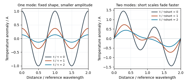
Original diffusion solutions: one Fourier mode loses amplitude, and a two-mode profile loses its short-wavelength structure faster
. Details. 
Write . For , direct partial differentiation givesHence exactly when , proving the claimed diffusion equation solution. At , , so . The infinite spatial domain needs no end-boundary conditions. For positive thermal diffusivity the amplitude decreases, as described by the thermal diffusion rate of a Fourier mode.
For a constant-mass, well-mixed box the mean residence time is stored water mass divided by its total outgoing water-mass transport. Using the source figure’s endpoints,At water steady state, each denominator can equivalently be replaced by that box’s summed inflow. If transports are specified as volume rates, use volume rather than mass in the numerator, or convert with density consistently. The drawn maximum basin depths alone do not supply layer volumes, plan areas or transport magnitudes, so no numerical residence times follow. Internal recycling counts as exit from a particular box; these times are not the time to escape the combined sea system.
There are unlisted articles, also show them or only show them.