
A Hermitian matrix has . ChooseIts off-diagonal entries are complex conjugates and its diagonal entries are real, so the defining condition holds. It is also invertible.
A symmetric matrix has , without conjugation. One invertible example with nonreal off-diagonal entries isIt is symmetric but not Hermitian, illustrating the importance of the distinction over .
For , maximize to lower the quartic coefficient. The identity shows that its maximum occurs for . ThereforeThere are eight symmetry-related easy directions. This is a cubic easy-axis anisotropy even though the selected directions are body diagonals; it is not a continuous easy plane. At the quartic free energy instead has a sphere of degenerate orientations to this order.
For , minimize the nonnegative anisotropy invariant . Its minimum is zero, achieved only when one squared component of the unit vector is one and the others vanish. Thus the easy directions areThe six signs and axes are symmetry-related ferromagnetic domains. Allowing the magnetization amplitude to relax does not change the result: its minimum free-energy reduction is proportional to , which is most negative for the smallest positive quartic coefficient. A direction has and is not an equally stable easy direction.
Child Created 2026-10-25 Updated 2026-11-05
Adolescence Created 2026-10-25 Updated 2026-11-05
A developmental period spanning changes in physical maturation, social roles and increasing autonomy. Clinical research should specify sampled ages and relevant developmental characteristics rather than treating an age label as a complete explanation of treatment response.
SU(N) fundamental completeness relation Created 2026-10-25 Updated 2026-11-05
For traceless Hermitian matrices representing the Lie algebra of the special unitary group , normalized by , completeness of in the space of Hermitian matrices gives the displayed identity. In particular . For traceless , this becomes . These identities reduce QCD color charge sums without choosing explicit matrices.
For the special unitary group , put . Its defining representation has weight system , and its exterior square has weight system ; each has multiplicity one. Their dual representations negate the weights of a representation. The Dynkin label coordinates are . These follow by evaluating diagonal traceless generators on coordinate vectors and their exterior products.
Under the standard embedding , the last defining weight of a representation restricts to zero and the others become the defining weights of a representation of . Splitting pairs according to whether they contain the last index proves the branching of a representation and , including multiplicities.
Identical-pulse Ramsey return probability Created 2026-10-25 Updated 2026-11-05
For ideal identical pulses separated by , multiply the unitary operators to obtain . An input at either pole of the Bloch sphere returns to that same pole with probability . In particular zero delay gives a full NOT, so its return probability is zero. Opposite-sign pulses instead give . The distinction matters when identifying the measured quantum state population.
A geostationary orbit is a circular, prograde, equatorial orbit with period equal to one sidereal day, approximately . Its satellite therefore remains above one longitude on the equator. Merely having a one-day period gives a geosynchronous orbit; an inclined or eccentric version still moves across the ground observer's sky.
Balancing gravitational acceleration and centripetal acceleration givesOne route is injection into an elliptical geostationary transfer orbit, followed by a burn near apogee to circularize and remove the remaining inclination; direct or low-thrust transfers are also possible. Subsequent station keeping controls longitude, inclination and eccentricity.
The fixed wide view permits frequent observations of weather, clouds and rapidly changing storms, as in Meteosat and GOES. The tradeoffs are large range, generally coarser spatial sampling for comparable optics, oblique views at high latitudes and poor polar coverage. It is valuable for following change through the day rather than obtaining global coverage with one spacecraft.[ref]
Catalog of Earth satellite orbits by NASA Earth Observatory. “High Earth Orbit”: geosynchronous radius, the circular/equatorial conditions for geostationarity, and weather-monitoring applications.
A Sun-synchronous orbit maintains approximately constant orientation relative to the mean Sun, so corresponding passes over a location occur at nearly the same local solar time. It is usually a nearly polar, slightly retrograde low Earth orbit. Earth rotates beneath the successive tracks, allowing broad coverage; the satellite is not stationary over a location and does not necessarily revisit that location every day.
It is attained by selecting altitude, orbital eccentricity and orbital inclination so that nodal precession caused by Earth's equatorial bulge matches the mean apparent annual motion of the Sun, about per year eastward. To leading order,Here is the semi-major axis, the orbital eccentricity, the orbital inclination, the mean motion, and Earth's dimensionless quadrupole coefficient. A retrograde inclination has , giving the required positive precession; typical imaging altitudes yield inclinations around –. The launch establishes the required orbital plane, and subsequent orbit maintenance limits drift.
This geometry suits repeated optical and multispectral imaging of land, vegetation and oceans, because comparable local time reduces illumination and shadow differences. Landsat and Sentinel-2 are examples. Radar missions such as Sentinel-1 also use this orbit for regular global sampling even though their illumination is supplied by the radar. Constant local time helps comparison but does not remove seasonal changes in solar elevation.[ref]
Catalog of Earth satellite orbits by NASA Earth Observatory. “Polar Orbits” and “Sun-Synchronous Orbits”: near-polar global sampling and controlled precession maintaining local solar time.
Pore fluid pressure reduces the compressive load carried across grain contacts or an accessible fault. In the usual elementary approximation,At fixed total stress, increasing translates the entire Mohr circle left by without changing its radius or the differential stress. The circle therefore approaches the frictional failure envelope even though the applied shear has not increased. Equivalently, in total-stress coordinates the strength on an existing plane is , reduced by . For a known orientation and constant frictional parameters, the ideal critical pressure isprovided the plane is in contact and sliding failure is reached before tensile opening.
For the diagram's illustrative , , and , the dry circle is below failure. The freely oriented tangency threshold is about ; the circle is already beyond that threshold and shows the loading tendency, not a stable post-failure state. If grows enough that , fluid pressure can instead open a tensile fracture. A porous-continuum effective stress law may use with a coefficient different from one. Also, changing fluid pressure can change total stress through constrained deformation; pure horizontal translation assumes those total stresses remain fixed.[ref]
Stress and strength lecture notes by MIT OpenCourseWare. Lecture 10, frictional strength modified by pore-fluid pressure.
Draw a failure envelope in the plane. A useful brittle shear-failure approximation is the Mohr-Coulomb failure criterionwhere is cohesion, the internal friction angle, and the effective compressive normal stress. A circle wholly inside the envelope is below this ideal failure threshold. Increasing the differential stress expands it until it first touches the envelope: the tangent points identify the failing plane orientations. For a linear envelope, tangency impliesWith the angle convention above, the upper tangent point is at . Its plane therefore makes with the maximum-compression direction; there is a conjugate plane on the other side. For , this is , rather than the plane of maximum shear stress. An existing weak fault can reactivate first, with its own lower cohesion and friction, and need not have this optimum new-fracture orientation.
For tensile brittle fracture, add a tensile strength cutoff: failure occurs when , where . The opening fracture is approximately perpendicular to the minimum-compression direction. Real rock envelopes curve, especially at small confinement; a straight shear envelope must not be extrapolated as an exact tensile law. High confinement can instead favor distributed or ductile deformation, so merely drawing a larger circle does not establish that brittle failure is the active mechanism.[ref]
Stress and strength lecture notes by MIT OpenCourseWare. Lecture 10, frictional strength and Mohr construction; the tensile cutoff is a separate condition.
For a plane whose normal lies in the – plane, rotate through from in the stated sign convention. The circle point givesThe normal-to-plane angle is essential: if the angle supplied is between the plane itself and , use its complement for . The principal stress planes have zero shear stress, and planes at to those principal stress planes have maximum .
For an arbitrary plane in a fully three-dimensional stress field, let be its direction cosines in the principal stress basis. ThenThese follow by resolving the traction into its normal and tangential components; the compression-positive tensor is the negative of the usual tension-positive Cauchy stress tensor. The family of Mohr circles visualizes the possible combinations, but the two-dimensional rule alone does not specify an arbitrary three-dimensional orientation.[ref]
Near the south magnetic pole, the inducing magnetic field and induced magnetic moment are vertically upward. Directly over the car its dipole field is also upward, again reinforcing the main field. The total-field magnetic anomaly is therefore the same positive central high and weak negative side lobes as at the north magnetic pole under the same induced-dipole assumptions. A fixed signed vertical field component would reverse, but the scalar field strength measured by the proton-precession magnetometer does not. If the car's remanent magnetization dominates, neither this symmetry nor these predicted signs is assured.
At the magnetic equator, the inducing magnetic field and induced magnetic moment are horizontal. Let point along this field, approximately magnetic north, and across it. Directly over the car, the dipole field opposes the main field, producing a negative central total-field magnetic anomaly. A north–south traverse through the car givesa symmetric central low with positive shoulders. An east–west traverse through the car instead has , a single negative trough. The equatorial anomaly therefore needs a stated traverse orientation; there is no universal single equatorial line profile.
Near the north magnetic pole, take the inducing magnetic field and induced magnetic moment as vertically downward. Directly above the car, its anomalous field reinforces the main field: a positive central total-field magnetic anomaly results. Along a horizontal traverse, the vertical-dipole approximation gives a symmetric central high flanked by weaker negative side lobes:where is the depth from the sensor to the effective dipole centre. The anomaly width scales with ; no absolute amplitude can be calculated without the car's magnetic moment.
For the fully gas-filled reservoir,soBoth impedances are now smaller than those of the cap rock. Both reflections reverse seismic reflection polarity, with a substantially larger amplitude for the P wave reflection. Reading the right-hand endpoint instead as would give , preserving the interpretation.
For the fully water-filled reservoir, the approximate densities and wave speeds giveand henceBoth are positive: the reservoir has larger P wave and shear-wave impedances than the cap rock, and neither reflection reverses the chosen stress-wave seismic reflection polarity.
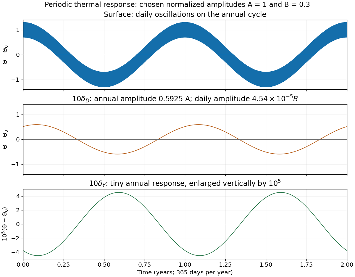
At , the annual attenuation is and the daily attenuation is , approximately . ThusOn the same vertical scale as the surface plot this is almost the constant . With a sufficiently enlarged scale, a residual annual oscillation of amplitude remains. Its phase lag is ten radians, interpreted modulo when comparing periodic maxima.

There are unlisted articles, also show them or only show them.