
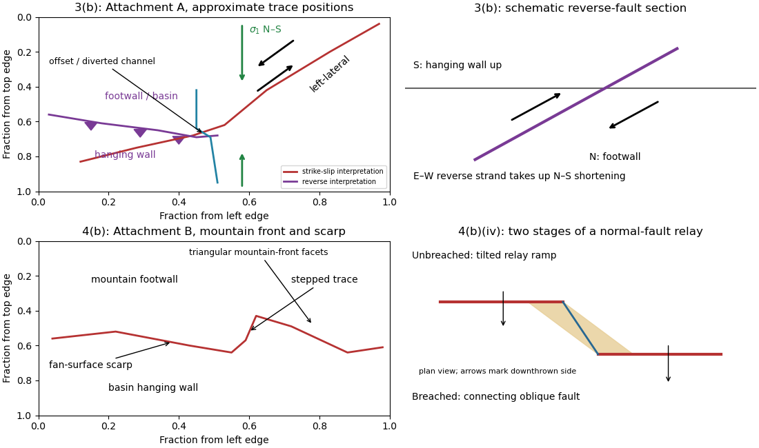
An overlapping pair of basin-dipping normal fault segments can first accommodate displacement through an unbreached relay ramp. Fault throw tapers toward each tip and transfers between the strands; the intervening block tilts and bends while retaining a continuous ramp-like surface. Draw overlapping parallel traces in plan view and a tilted connecting surface between their different fault throws.
With continued extension, the ramp can be breached by a linking fault. An oblique connector joins the segment tips and takes up a combination of dip-slip and strike-slip displacement; the system becomes a more continuous, zigzag normal fault. Draw this connector diagonally through the overlap, with downthrown arrows on the basin side. Distributed small faults and folding can accompany either arrangement. The central bend around in Attachment B is the candidate transfer zone; the image alone does not uniquely establish the three-dimensional connection at depth.
The rate of surface modification controls how quickly a fault scarp is erased. Strong rainfall, runoff, slope failure and easily eroded lithologies can round or dissect a scarp; dry conditions and resistant rock often preserve it longer. Alluvial fan deposition and aggradation can bury a scarp even if erosion is slow. A young marker surface can preserve an offset that an older, strongly modified surface no longer records.
The balance between fault slip rate, recurrence interval and marker age controls whether renewed displacement outruns this modification. Rapid or repeated normal faulting can maintain a clear front, whereas a long interval after a small displacement permits smoothing. A very young fan deposited after the event may have no offset, while an older surface may retain cumulative rather than single-event fault throw. These two controls explain why absence of an obvious scarp is not proof of an inactive fault.
Mark a fault scarp cutting an alluvial fan on the left-to-central smooth piedmont, approximately . Its narrow, aligned height break continues across surfaces that are smoother than the mountains; repeated downthrow on the basin side produces the scarp. Sketch a once-continuous gently sloping fan surface cut by a basin-facing step.
Mark triangular facets on the mountain front in the right-central part, near . These are roughly triangular planar mountain faces bounded laterally by incised valleys and below by the fault front. In a front view, draw repeated triangles separated by stream valleys. Triangular facets result from the interaction of normal faulting, uplift and erosion; neither they nor a sharp mountain front alone demonstrates a rupture in the particular historical event.
Map the continuous break near the base of the rugged mountain front, following the low scarp across the smoother fan surfaces, rather than the ridgeline. With the same normalized image coordinates, an approximate trace follows , steps toward , and continues via . Some parts are much clearer than others and should be drawn as inferred or dashed where obscured.
The mountainous upper side of the image is the uplifted footwall; the smoother basin/fan side below is the downthrown hanging wall. A section perpendicular to the front has a normal fault dipping toward the basin. Attachment B has no printed north arrow, so these image-relative labels avoid assigning an unsupported compass direction. The original interpretive figure marks the trace and the central fault step-over.
The network partitions deformation into oblique horizontal displacement on the strike-slip fault and more directly north–south crustal shortening on the approximately east–west reverse fault. On the oblique strand, northeastward motion of the southeastern side relative to the northwestern side has a northward component, reducing separation in the direction of . On the reverse fault, northward and upward motion of the southern hanging wall shortens and thickens the crust.
Sketch north–south opposing compression arrows around the plan view, left-lateral arrows along the oblique trace, and teeth on the southern side of the reverse fault trace. A section normal to the latter shows horizontal shortening converted into tectonic uplift. Where strands meet, folding, distributed strain or subsidiary faulting can maintain displacement compatibility; a strike-slip fault terminating abruptly in undeforming rock would not. This is an interpretation involving transpression, and the map does not by itself give a unique partition of slip rates between the strands.
Put the reverse fault along the mountain-front trace identified in part (ii), with the mountainous southern/southwestern block as hanging wall and the central basin to its north/northeast as footwall. Draw teeth on the southern hanging wall side of the line. In the simplest cross-section the fault dips south and the southern block moves northward and up over the basin edge. The image constrains the surface trace and relative uplift more securely than its subsurface fault dip; the precise dip cannot be measured from this map alone.
Trace the strike-slip fault along the southwest–northeast valley, approximately through . The long oblique strand is interpreted as left-lateral strike-slip faulting: draw the southeastern side moving northeast and the northwestern side moving southwest, parallel to the trace.
This sense is consistent with horizontal north–south maximum compression: for an approximately northeast-striking fault, the resolved shear stress moves the southeastern side northeastward relative to the northwestern side. The deflected central drainage supports that interpretation. The regional stress direction supplies a consistency check rather than a uniquely precise trace location; follow the geomorphic break rather than drawing a single straight line through every coordinate.
A reverse fault can create a sharp mountain front by raising its hanging wall beside a lower footwall. Drainages entering the rising block may be deflected along the front or cut narrow gorges across it. In cross-section, draw a dipping fault with the hanging wall displaced up-dip and a surface-height contrast above the trace.
In Attachment A, mark the approximately east–west to west-northwest–east-southeast break between the southwestern mountain block and the central basin. Its approximate image coordinates run from through and to . The abrupt topographic change and diversion of drainage along this front support the reverse faulting interpretation. It is the southern margin of the central basin, not the much straighter oblique valley farther northeast. The original interpretive figure gives a schematic section.
A displaced drainage forms when repeated horizontal fault slip offsets a channel and its upstream and downstream reaches no longer line up. In plan view, draw two initially continuous channel reaches crossing the fault, translate one side parallel to the fault strike, and connect the reaches by a short fault-parallel reach. A linear valley develops where erosion follows damaged rock along a straight fault zone.
In Attachment A, use the oblique, relatively straight valley running southwest–northeast through the lower centre towards the upper right. For an identifiable example, follow the central approximately north–south drainage to its bend near the southern edge of the central basin, about , where is fraction from the left image edge and fraction from the top. Mark its deflected reach and the adjacent straight valley. The positional precision is at the level of the supplied image; establishing a numerical fault offset would require correlated piercing points and field checks.

For , direct differentiation again gives and . Thus it satisfies the heat equation. Moreover,vanishes at both endpoints for integer , proving the homogeneous Neumann boundary conditions. Now gives the nonzero constant mode , which does not decay. It represents conserved mean temperature in an insulated plate.
Put and . Direct differentiation of givesso , the heat equation. At , the sine factor vanishes; at , it is for integer . Thus the homogeneous Dirichlet boundary conditions hold. The nonzero, nonredundant spatial modes use ; is the zero function and negative only change the amplitude sign.
By Fourier's law, . With nonzero thermal conductivity , zero outward heat flux at both endpoints gives homogeneous Neumann boundary conditions:The outward normal has opposite signs at the two ends, but a zero-flux condition gives zero derivative at each.
For , fixed zero endpoint temperatures are homogeneous Dirichlet boundary conditions:An initial condition is also needed to determine a particular solution of the heat equation.
First measure the generator’s spectrum, timing and propagation pattern on quiet records. If practicable, coordinate shutdowns or quiet acquisition windows; otherwise place source/receiver lines to reduce coupling to the noise source and use good ground coupling and adequate instrument dynamic range. Saturated channels cannot be repaired by a later filter.
Separate noise using its measured frequency and moveout: a band-pass/high-pass filter can reject frequencies below the useful seismic band, and an appropriate narrow notch can reject a narrow coherent component. Avoid deleting wanted low-frequency arrivals along with the generator noise. Dense spatial sampling enables frequency–wavenumber filtering or array methods to separate low-apparent-velocity surface noise from target arrivals. A reference sensor near the generator can support coherent-noise subtraction when the transfer is stable.
Repeated shots/sweeps and stacking improve the signal-to-noise ratio for uncorrelated noise; persistent coherent generator noise does not necessarily average down. Known-sweep Vibroseis correlation also helps reject unrelated noise. Verify the final processing against test gathers to ensure that real arrivals have not been mistaken for noise.
Choose shot and receiver intervals to sample the shortest relevant spatial wavelength and steepest event moveout without spatial aliasing. A simple bound isusing the smallest apparent velocity of the events one needs to retain or separate. Using and Hz alone suggests m, but slower surface waves or dipping events can demand finer spacing. It is not a universal final design interval.
Also consider target depth and lateral resolution, reflector dip, near-surface heterogeneity, source strength and coupling, maximum offset and aperture, common-midpoint bin size and seismic acquisition fold, refraction crossover distances, access and budget. Receiver spacing and source spacing jointly determine coverage and cannot be selected from temporal sampling alone.
The Nyquist–Shannon sampling theorem gives a Nyquist rate of samples per second for a Hz upper frequency. In practice choose Hz, for example Hz with ms, and use an anti-aliasing filter whose passband retains the required signal below the Nyquist frequency. Exactly Hz leaves no filter transition band and can entirely miss a Hz sinusoid at an unfortunate phase; it is a limiting rate, not a robust acquisition choice.
At each source position, couple the vibrator to the ground, transmit a known frequency sweep and record the ground response on synchronized geophones. Record a pilot or measured source-force reference and sufficient listening time for delayed arrivals. Repeat sweeps where beneficial and retain geometry and timing information.
If the Earth’s impulse response is , a linear model is . Vibroseis correlation cross-correlates the record with the known sweep:The sweep’s autocorrelation is a compact, approximately zero-phase wavelet, so the long chirp is compressed into identifiable delayed events. In the frequency domain this multiplies by , yielding plus noise. It is pulse compression, not an exact recovery of at frequencies never transmitted. Spectral shaping or stabilized deconvolution can further compensate the finite source bandwidth and sidelobes.[ref]
Geophysical Survey Summary Report, Section 3: Geophysical Testing Methodology. Vibratory sources: known input sweep correlated with geophone records
An explosive seismic source gives an impulsive, potentially high-energy broad-band signal and can couple effectively to competent material. It can be useful where strong penetration is needed and heavy vibrating vehicles cannot reach the site. Disadvantages include destructive ground disturbance, permitting and specialist handling, variable source coupling and signature, and the cost of repeated source preparation. The comparison does not require a prescription for charge size or emplacement.
Vibroseis spreads controlled energy over a longer frequency sweep. It is repeatable, permits tailored bandwidth and repeated sweeps, and its known signal supports correlation processing and rejection of unrelated noise. It avoids the impulsive ground disruption of an explosive source. Disadvantages include vehicle access and terrain restrictions, dependence on baseplate coupling, limited force and low-frequency performance, possible harmonic distortion, and strong near-surface waves. For a fractured shallow geothermal site, test which source produces usable coherent reflections or arrivals in the desired band; nominal source energy alone does not establish data quality.
Specify the amplitude convention. For normal-stress/pressure amplitudes, the seismic reflection coefficient and seismic transmission coefficient areFor particle displacement or velocity resolved in one fixed normal coordinate, the reflected amplitude changes sign and the transmitted ratio is insteadThese are alternative conventions, not conflicting energy predictions. The reflected and transmitted energy flux fractions arewhich sum to one for the ideal lossless interface. Thus an amplitude transmission coefficient greater than one does not violate conservation of energy.
The normal-incidence acoustic impedance is . ThereforeThese are and MRayl. They combine the material’s density and wave speed; using would give shear rather than acoustic P impedance.
There are unlisted articles, also show them or only show them.