
Past exam of the symmetry and relativity course of the University of Oxford 2016 4 c a Solution 2026-10-25
An isolated free electron in vacuum cannot spontaneously emit a nonzero real photon. If , where is the emitted photon four-momentum, and , conservation would require . A future-pointing timelike four-vector has strictly positive inner product with every nonzero future-pointing null four-vector, so this is impossible.
The same conclusion follows from the classical Cherenkov radiation condition : in vacuum , while the electron with has . Hence there is no vacuum emission angle for the specified free particle. Acceleration by an external field or scattering from another body would change the physical problem and can permit radiation.
Past exam of the symmetry and relativity course of the University of Oxford 2016 2 c b Solution 2026-10-25
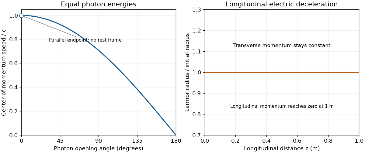
The center-of-momentum frame moves with velocity . Using the total four-momentum in solution givesFor , its direction bisects the two photon directions, and its speed decreases from the limiting value to zero. At , the lab already is the center-of-momentum frame. At , the formal speed is and no inertial rest frame exists; this endpoint is a limit, not an allowable boost.
Past exam of the symmetry and relativity course of the University of Oxford 2016 2 c a Solution 2026-10-25
Each photon has energy . Their total four-momentum isIts squared invariant is . Therefore the system's rest energy isTwo individually massless particles can thus have positive total invariant mass. Back-to-back photons give rest energy , whereas exactly parallel photons have zero invariant mass and no massive-system rest frame.
Past exam of the symmetry and relativity course of the University of Oxford 2015 4 b iii Solution 2026-10-25
Write . Substituting into ii gives . The positive-separation branch therefore hasThe Born-rigid front trajectory from a rear worldline follows by setting :Every and in this formula is evaluated at the rear event with laboratory time , not at the shifted argument of .
For completeness, a smooth future-directed front trajectory requires this time mapping to be locally invertible. If the signed laboratory acceleration is and the rear proper acceleration is , thenWhen , their ratio gives , so the two simultaneous points indeed share their instantaneous velocity. If that factor reaches zero, an acceleration-horizon obstruction appears; an arbitrary rear trajectory cannot be extended to an arbitrary rigid length while retaining both rockets future-directed. The positive-acceleration example below satisfies the condition.
Past exam of the symmetry and relativity course of the University of Oxford 2015 4 b ii Solution 2026-10-25
Use the same event pair already made simultaneous in the rear instantaneous rest frame. Its proper spatial separation is the Minkowski interval length, soThe inequality selects the front rocket rather than the equally long backward extension. Equivalently the Lorentz-transformed spatial difference obeys . This is not the condition at equal laboratory times, which would describe the stretching arrangement in a.
Past exam of the symmetry and relativity course of the University of Oxford 2015 4 b i Solution 2026-10-25
Let on the rear rocket and on the front rocket. The instantaneous inertial rest frame of the rear rocket at moves at relative to S. Transform the time difference of these two events:Setting givesThe velocity belongs to the rear event . It is not to be evaluated at laboratory time , nor does the simultaneity condition mean in S. At nonzero velocity the front event on the same instantaneous-rest slice is at a different laboratory time.
Past exam of the symmetry and relativity course of the University of Oxford 2015 2 c iii Solution 2026-10-25
Let the fixed direction of motion be the unit vector and decompose . In ii the two parallel contributions cancel, whereas the transverse equation isFor the stated speed law, , hence . Since the particle is initially at rest, , andThe corresponding spin four-vector has components , , and . Its squared norm is therefore , independent of time. The transverse decay of the source's laboratory three-vector is a boost-normalization effect, not a loss of proper angular momentum or a torque.
For a real increasing speed take and . The prescribed profile has a singular initial acceleration: near zero. The differential transport calculation applies for and the solution has the continuous initial limit displayed above. This trajectory should not be silently described as motion at constant proper acceleration.
Past exam of the symmetry and relativity course of the University of Oxford 2015 2 c ii Solution 2026-10-25
Take the dot here to mean , as in the source. Differentiate and the given spin components. Their contraction simplifies because the terms involving cancel:The spatial part of the transport equation consequently readsUse and divide by . The result isNo assumption of acceleration perpendicular to the velocity was made. In particular the second term cannot be dropped for a particle speeding up along a straight line. This is the three-vector in the source's particular spin four-vector parametrization; its Euclidean magnitude need not be the invariant proper-spin magnitude.
Past exam of the symmetry and relativity course of the University of Oxford 2015 2 c i Solution 2026-10-25
For the source's definition , direct contraction with givesIt remains zero under the torque-free transport law. Differentiate the contraction, using the product rule and :Thus an initially spatial spin in the instantaneous rest frame remains orthogonal to the velocity. This is the orthogonal-spin specialization of Fermi-Walker transport. The sign is tied to the negative timelike norm; using the opposite metric sign without changing the transport formula would spoil the cancellation.
Past exam of the symmetry and relativity course of the University of Oxford 2015 1 c v Solution 2026-10-25
Using the conventional critical scale rather than guessing a precise Fourier-width coefficient,This is extreme ultraviolet and the very soft X-ray boundary, with a broad spectrum extending on either side; it is not a hard, multi-keV X-ray source at the stated large bending radius. The characteristic energy is not a sharp upper cutoff. For orientation, the standard angle-integrated spectral power per unit frequency peaks near eV, also in the extreme ultraviolet; a particular angular acceptance weights that spectrum differently.
The crucial scale follows from both the GeV energy and the m radius. Using only the fact that synchrotron sources can make X-rays, or replacing the bending radius by a much smaller unstated value, would misidentify the characteristic photon energies here. The critical-energy convention and the broadband character are described by the primary radiation model.[ref]
Synchrotron Radiation in the Geant4 Physics Reference Manual by Geant4 Collaboration. photon-spectrum section, equation (209), and Properties of the Power Spectra
Past exam of the symmetry and relativity course of the University of Oxford 2015 1 c iv Solution 2026-10-25
A shorter radiation flash has a broader Fourier transform. From iii, its characteristic angular-frequency bandwidth isAt fixed bending radius this scales as as . The standard synchrotron critical angular frequency makes the same scaling explicit:A periodically circulating electron produces harmonics of its revolution frequency. The very large harmonic range, of order , forms the familiar effectively continuous broad synchrotron spectrum at ordinary detector resolution. The result concerns the intrinsic spectrum of the radiation, not merely the slow envelope imposed by a long incoherent bunch. Ordinary frequency is ; mixing cycles per second with radians per second would introduce a spurious factor of into photon-energy estimates.[ref]
Synchrotron Radiation in the Geant4 Physics Reference Manual by Geant4 Collaboration. critical-energy formula and validity discussion, critical harmonic number
Past exam of the symmetry and relativity course of the University of Oxford 2015 1 c iii Solution 2026-10-25
A fixed distant observer receives appreciable radiation while the velocity points within an angle of order of the line of sight. The corresponding emission interval is . The source moves toward the detector during that interval, shortening the light-travel distance. In the far-field limit,where is the angle between velocity and the detector direction. Near the tangent, , soThe emission interval itself is of order s. Omitting the arrival-time compression would therefore miss many orders of magnitude.
For a definite angular window , integrating the arrival-time relation givesThe order-one coefficient depends on how the beam window or pulse width is defined. These are intrinsic single-electron radiation-flash scales. For bunch-length broadening of synchrotron radiation, a finite bunch moving through the same tangent point contributes an arrival-time spread of order its length divided by ; the longitudinal bunch profile and instrumental response must be convolved with the intrinsic flash. “Short bunch” alone does not specify an experimental bunch pulse duration at the attosecond scale, because no bunch length has been supplied.[ref]
Synchrotron Radiation by Richard Fitzpatrick. §12.22, equations (1974)–(1981), beaming and arrival-time compression
Past exam of the symmetry and relativity course of the University of Oxford 2015 1 c ii Solution 2026-10-25
Relativistic relativistic aberration concentrates emission into an angular scaleThis is a half-angle or characteristic divergence scale; a full cone opening is about twice it. The exact half-photon-count cone in a applies to isotropic rest-frame emission. A synchrotron emitter has its own rest-frame angular radiation pattern, so that count result should not be treated as an exact median-power formula for the synchrotron beam. It nevertheless gives the correct relativistic beaming scale. Electron-beam emittance, vertical angular spread and the detector's acceptance can broaden the experimentally observed divergence beyond this intrinsic estimate.
Past exam of the symmetry and relativity course of the University of Oxford 2015 1 c i Solution 2026-10-25
Interpret GeV as the electron's total energy; the alternative kinetic-energy reading changes the estimate only slightly at this scale. The Lorentz factor and orbital acceleration areUsing the supplied Larmor formula, and the revolution time ,For m this gives W per electron and s. Their product isThis is the energy loss of one electron on a full circular orbit, not its energy loss per metre or the total loss of the whole bunch. The fractional loss is only about of the GeV energy each revolution. Maintaining a steady stored energy requires replacing that energy through the accelerator's rf system.
Past exam of the sub-atomic physics course of the University of Oxford 2016 2 c c Solution 2026-10-25
The beam energy is a total pion energy, so the momentum follows the relativistic relation . Taking the standard charged-pion rest energy MeV,[ref]For motion perpendicular to a uniform magnetic field, the Lorentz force supplies the transverse momentum change and gives . With the stipulated eV s m,The unit cancellation leaves length after dividing by in metres per second. Equivalently, the usual magnetic-rigidity conversion is for unit charge. The sign of the pion charge chooses the bending direction, while the radius uses its magnitude. Treating the pion as massless would give about m and is not a good approximation at this modest total energy. The production target does not determine the downstream orbit once the pion momentum and magnetic field are specified.
Past exam of the sub-atomic physics course of the University of Oxford 2016 2 c b Solution 2026-10-25
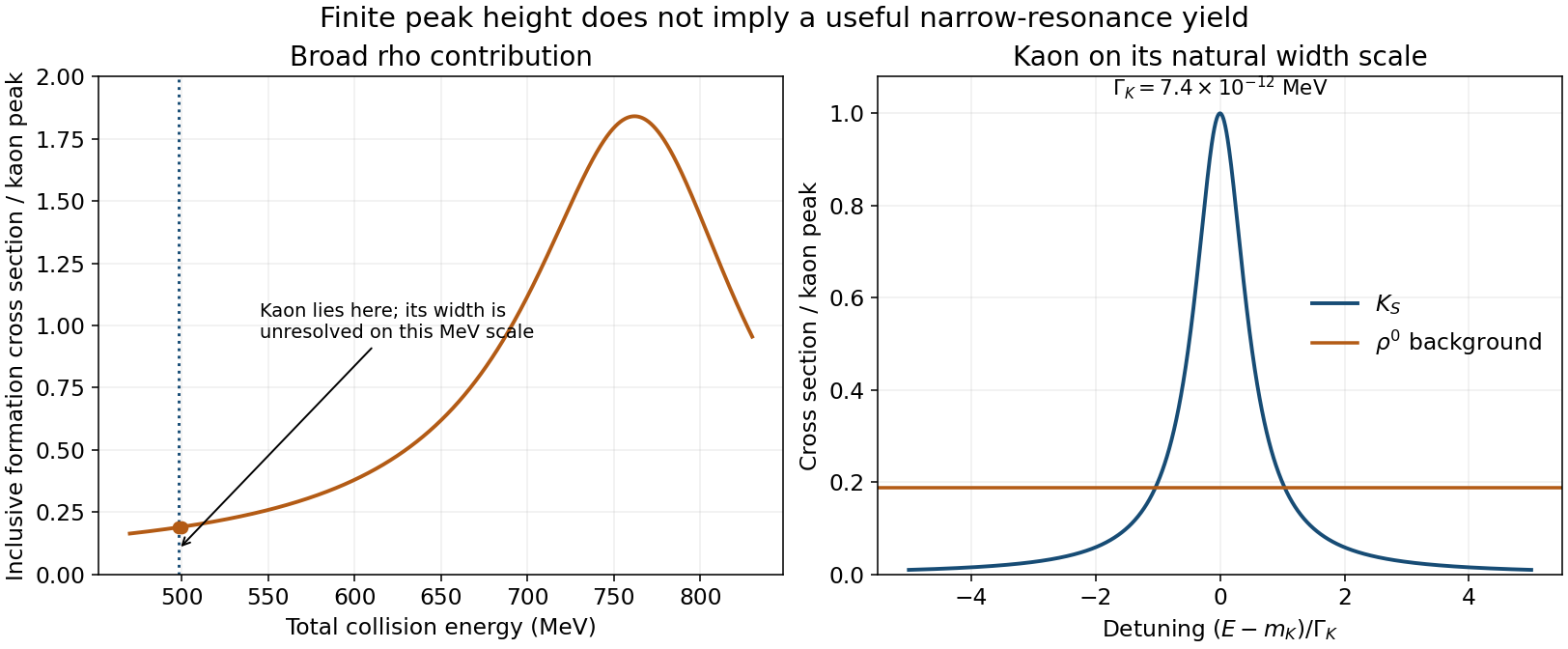
Raising each beam energy to 250 MeV makes MeV. The kaon denominator is now dominated byrather than by . Substituting into a givesThe enormous change is a tiny-width effect, not a comparably abrupt change in the broad rho contribution. The center-of-momentum energy has moved about kaon widths from the peak. A width of MeV is only eV, requiring an energy-selection scale of order relative to the several-hundred-MeV beam energy.
Real beams have vastly broader energy distributions. Averaging over such a distribution suppresses the useful narrow-resonance contribution: the finite peak value does not imply a large energy-integrated formation rate, whose resonant area shrinks with the width at fixed branching fractions. The weak inverse-decay entrance coupling and the broad strong-interaction rho background therefore make this a poor way to study kaon resonant formation. The supplied broad-resonance formula is used algebraically as requested; a practical calculation would convolve an appropriate narrow line shape with the actual beam distribution.


Past exam of the sub-atomic physics course of the University of Oxford 2016 2 c a Solution 2026-10-25
Use and let denote the total center-of-momentum energy, not one beam's energy. Opposite equal momenta give MeV, so the kaon is at its stipulated resonance mass MeV. Write the unspecified selected exit branching fractions as and . The supplied line shape givesThe distinction between inclusive and exclusive resonance branching factors matters here. For inclusive resonance formation, sum over all decays, so . At the small kaon width cancels from the peak value:If instead the measured cross section is specifically resonant elastic , its exit branching fractions equal the entrance ones: , . ThenThe source says production without specifying an observed decay channel, so both conventions are made explicit rather than silently squaring a branching fraction for an inclusive measurement. The quoted kaon width and two-pion branching fraction identify the short-lived propagation state ; a pure flavor state is a superposition of short- and long-lived states. This exercise uses the stipulated resonance model and equal omitted proportionality factors.
Past exam of the sub-atomic physics course of the University of Oxford 2016 1 b c Solution Created 2026-10-25 Updated 2026-11-05
Adding the three characteristic quark energies from b givesThe estimate recovers a sub-GeV scale but underestimates the stated neutron mass by a factor of a few. This is consistent with its deliberately crude uncertainty and geometry assumptions; it is not a precision mass prediction.
A better model needs the actual spatial and momentum correlations, a confining interaction, and the energy in the quark and gluon fields. In quantum chromodynamics, hadron masses are not simply the sum of three freely moving particles with tiny masses. The supplied MeV rest-energy scale resembles a light current-quark scale; a phenomenological constituent-quark mass includes substantial dressing and is a different parameter. Color, spin correlations, relativistic dynamics and sea components all matter when defining a more realistic bound-state Hamiltonian operator or performing a lattice QCD calculation. The prescribed uniform-sphere model supplies none of those extra dynamical inputs, so its discrepancy should not be repaired by an unannounced change of the given radius or mass.
Past exam of the sub-atomic physics course of the University of Oxford 2016 1 b b Solution 2026-10-25
Adopt the lower-bound scale of the Heisenberg uncertainty principle, , with the prescribed radial scale from a. Using MeV fm,For a one-sided exponential distribution of a positive momentum magnitude, , both its mean and its standard deviation are . Under the additional identification made in this estimate, set the characteristic momentum to . This identification concerns a positive magnitude; the mean of a signed momentum component in an isotropic stationary state would instead vanish.
Use the relativistic energy-momentum relation, not a nonrelativistic kinetic-energy approximation, because the momentum-energy scale is much larger than the stipulated quark rest energy:This is a characteristic energy estimated at the characteristic momentum. It is not an exact evaluation of over a fully specified three-dimensional wavefunction. An order-of-magnitude convention would give an answer about twice as large; the uncertainty principle by itself specifies a bound, not a unique confinement energy.
Past exam of the sub-atomic physics course of the University of Oxford 2016 1 b a Solution 2026-10-25
Uniform probability per volume does not give a uniform radial distribution. A shell of radius and thickness occupies volume , so the radial probability density function isIt integrates to one. The second radial moment isThe radial uncertainty scale in a uniform sphere supplies the position-uncertainty scale as instructed by the toy model. It is not literally the standard deviation of the scalar radius: and . Nor is a uniform spatial probability density sufficient to determine a unique momentum space wavefunction. This explicit distinction keeps the order-of-magnitude assumption separate from a fully specified quantum bound-state calculation. Replacing the radial density by a uniform density in would give a different second moment because it omits the spherical volume element.
There are unlisted articles, also show them or only show them.