
Past exam of the topics in fluid mechanics course of the University of Oxford 2023 2 a i Solution 2026-10-25
Take vertically upward and the porous skeleton stationary. Darcy's law and incompressibility areHere is the Darcy velocity, a volume flux per unit total cross-sectional area, including solid and void. If is the liquid pore velocity and all the pore space is saturated and connected, thenThe porosity therefore enters storage and the conversion to pore velocity; it does not multiply the Darcy velocity again when calculating discharge.
Past exam of the topics in fluid mechanics course of the University of Oxford 2023 1 b ii Solution 2026-10-25
Define . The linearization about givesThe Galilean transformation , has and . It removes the leading advection, leavingFor a normal mode proportional to , the second and fourth derivatives contribute and . The dispersion relation is thereforeFor and , the unstable wavenumbers satisfy . In the laboratory coordinates, the temporal exponent is , so this linear stability calculation predicts growth together with downslope transport at dimensionless speed .
Past exam of the topics in fluid mechanics course of the University of Oxford 2023 1 b i Solution 2026-10-25
For an inverted falling film, keep directed from the solid into the liquid. The downslope component of gravity is unchanged, but its normal component is now positive. Thus the hydrostatic pressure changes from to . The resulting Benney equation isOnly the normal-gravity contribution changes sign; the surface tension and inertial contributions retain their signs.
Past exam of the topics in fluid mechanics course of the University of Oxford 2023 1 a iv Solution 2026-10-25
Use an asymptotic expansion at fixed , evaluating the boundary conditions at the instantaneous . At leading order, the downslope equation gives . The wall condition and the surface condition implyHere denotes the total leading velocity, to distinguish it from the dimensional scale . The continuity equation and wall impermeability then giveThe transverse momentum equation gives . The normal stress condition therefore yieldsThe leading volume flux per unit width is . Consequently mass conservation gives . This relation eliminates inside the first inertial correction:Set . The downslope equation and boundary conditions areTwo integrations giveThe pressure correction is not needed for this calculation because its downslope pressure gradient enters only at .
Integrating the total velocity across the film givesIndeed the three inertial polynomial terms integrate to . Integrating the continuity equation and using the kinematic boundary condition gives . Hence the Benney equation isNormal gravity smooths height variations on the upper side of the slope, while the inertial correction can amplify them. Surface tension suppresses sufficiently short wavelengths.
Past exam of the topics in fluid mechanics course of the University of Oxford 2023 1 a iii Solution 2026-10-25
The two wall boundary conditions areDefine the capillary parameter for a falling filmRetain in the long-wave approximation. Thus surface tension is retained in the leading normal stress balance even though geometric slope corrections are small. For in the rescaled coordinates, the dimensional surface slope is .
The three free surface boundary conditions, accurate through , areThe first is the kinematic boundary condition; the second is the zero tangential traction condition. For the third, the dimensional liquid-side pressure is, to the required order,Division by gives in dimensionless variables. Subtracting gives the stated perturbation condition. The additional slope-times-shear contribution to normal stress vanishes at this order because the tangential traction is zero. The omitted geometric and tangential-stress corrections are under this ordering.
Past exam of the topics in fluid mechanics course of the University of Oxford 2023 1 a ii Solution 2026-10-25
Define the aspect ratio and the thickness-based Reynolds number byUse the nondimensionalizationThe small transverse velocity scale follows from incompressibility. Dropping stars, the base fields become and . Before subtracting the base state, the dimensionless Navier-Stokes equation readsFor example, division of the downslope momentum equation by makes the inertial coefficient and the pressure gradient coefficient . The transverse equation has been divided instead by after using its smaller velocity scale; this gives the displayed coefficient.
Now substitute , , . Since , , and the base fields have no or dependence, subtraction givesThese are nonlinear equations for the deviations; small amplitude has not been assumed. The later asymptotic expansion takes as , or more generally requires the retained inertial correction to remain small.
Past exam of the topics in fluid mechanics course of the University of Oxford 2023 1 a i Solution 2026-10-25
Take positive away from the wall into the liquid, and write for atmospheric pressure. For a constant-mass density Newtonian fluid, the two-dimensional Navier-Stokes equation and continuity equation areThe stationary wall imposes the no-slip boundary condition and no-penetration boundary condition, at . For a flat free surface with negligible air shear stress, the stress boundary condition is , at ; the kinematic boundary condition is there.
For steady flow independent of , these equations give , and . Two integrations and the boundary conditions give the uniform gravity-driven Newtonian film:Its surface velocity is , while its mean velocity is .
All daughter particles are massless, so the parent mass supplies the only kinematic scale at tree level. Each vertex has two derivatives, making its scattering amplitude scale as . For the four- vertex, symmetrizing over the derivative-bearing legs yields a sum of pairwise four-momentum products, which is proportional to by four-momentum conservation.
For massless daughters, the Lorentz invariance Lorentz-invariant phase-space measure scales as : each contributes two powers and the four-dimensional Dirac delta removes four powers. Including the parent factor gives . ThusThe unspecified factors are dimensionless angular integrals and identical-particle factors. Each result has mass dimension one, as a decay width must in natural units.
Counting the mass dimensions of each interaction operator givesIndeed and have dimension five, whereas has dimension seven. These are interactions of an effective field theory with dimensionful couplings.
The direct one-vertex decay channels are , and . Each leading scattering amplitude is linear in its corresponding coupling, and a decay width is quadratic in the amplitude. Therefore, holding the parent mass fixed,There are no tree-level interference terms between these different final states.
An hop can occur only while the charge occupies . Hence its stationary number per unit time isThe reverse count is , which equals this result. There is therefore no signed stationary current along that edge. The individual hopping traffic need not equal the contact-arrival traffic; their ratio is . A charge can make several internal visits before leaving, so neither conservation nor the single-charge constraint forces those two one-way rates to coincide.
Condition on the molecule being empty. Its instantaneous incoming-charge jump rate is , so the unconditional stationary number of arrivals per unit time isThis stationary jump traffic at a single contact is a unidirectional jump count, not a signed net current. Stationarity also gives . Multiplying their difference by the charge gives zero net stationary electrical current through the molecule's single contact, even though individual arrival and departure events continue.
Past exam of the symmetry and relativity course of the University of Oxford 2021 3 a ii Solution 2026-10-25
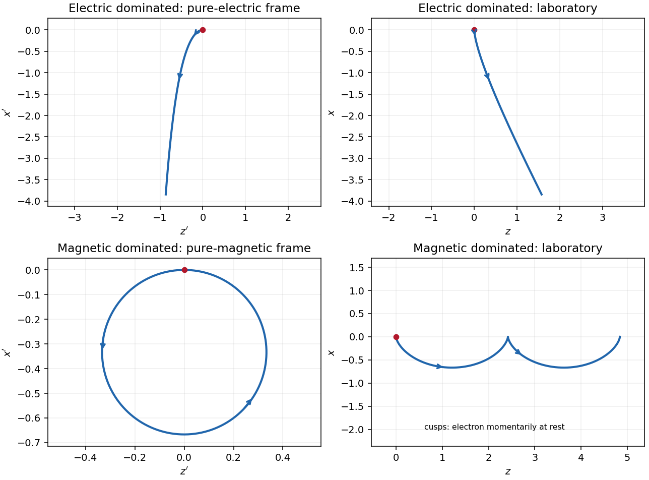
In the magnetic-dominated case the suitable Lorentz boost instead hasThe hypothesis gives . The electromagnetic field invariants now have , allowing a purely magnetic inertial frame. The initial velocity is again , perpendicular to . Since a magnetic field does no work, the electron's relativistic energy and speed in this inertial frame remain constant. Its trajectory is a circle in the plane with Lorentz factor and cyclotron frequency .
For , set and . A parametrization with the correct initial velocity and Lorentz force isTransforming the world line back to the laboratory givesThe laboratory trajectory is a stretched cycloid, with cusps at where the electron is momentarily at rest. It first accelerates toward , then curves toward , returning to its original coordinate each cycle while advancing in . Its mean drift is , the E-cross-B drift. Its laboratory kinetic energy oscillates as the electric field does positive and then negative work; it does not grow indefinitely. The strict inequalities in the two branches exclude the null case , where neither field can be removed by a finite Lorentz boost.
Past exam of the symmetry and relativity course of the University of Oxford 2021 3 a i Solution 2026-10-25
Assume for the directions and parametrizations; the boost formulas retain their signed meaning for reversed fields. A Lorentz boost with velocity along transforms the transverse electric field and magnetic field asIn the electric-dominated case chooseThe inequality ensures , so this is an inertial frame. The field-removing boosts for perpendicular electric and magnetic fields are governed by the electromagnetic field invariants and explain why a purely electric inertial frame exists and a purely magnetic one does not.
The electron is not initially at rest in this convenient inertial frame: its initial velocity is and its initial three-momentum is . Thereafter , while stays constant. The electric field accelerates it toward ; as its relativistic energy increases, its negative transverse velocity decreases in magnitude. Defining and gives a useful parametric world line:Here is the proper time. These formulas follow by integrating , , and constant . Its projection onto the plane is a hyperbola, but the spatial trajectory includes the initial transverse motion and is not a straight line.
Transforming back with , givesThe laboratory trajectory starts from rest toward , then bends toward . It is unbounded in and ultimately has and . Thus the late velocity has magnitude as a limit, consistent with the relativistic energy-momentum relation, rather than undergoing a closed cyclotron orbit.

Past exam of the symmetry and relativity course of the University of Oxford 2019 4 b ii Solution 2026-10-25
At atomic separations both massive exchange potentials are exponentially negligible. Molecular binding needs an interaction that survives at atomic distances; actual chemical bonds is governed principally by electromagnetism and quantum mechanics, with a massless photon rather than a scalar mediator. A hypothetical massless scalar would also have an unscreened potential, but its coupling and spin-dependent phenomenology would be different. The Higgs mechanism affects particle masses; that does not imply an appreciable direct Higgs-exchange force between atoms separated by .
Past exam of the symmetry and relativity course of the University of Oxford 2019 4 b i Solution 2026-10-25
A pion mass gives a Yukawa potential range of order a femtometre, so meson exchange can describe the short range of the residual nuclear force. The nuclear suppression relative to a massless potential of the same coupling is only about a factor of two at one femtometre. A Higgs-mass mediator instead has a range around and a further factor by nuclear separations; direct Higgs exchange cannot supply an appreciable long-range nuclear binding interaction at those separations. The range comparison does not replace the spin, coupling and many-body physics of actual nuclear forces.
Past exam of the symmetry and relativity course of the University of Oxford 2019 2 c iii Solution 2026-10-25
An excited-state population lifetime gives a natural linewidth whose Lorentzian full width in ordinary frequency iswhen no extra dephasing broadens it. Additional thermal motion, collisions or inhomogeneity may increase the effective width. Therefore excitation is appreciable over , rather than only at one event. A Lorentz line shape has nonzero wings, so is a line-centre threshold, not a mathematically sharp cutoff of all signal. Below it, only a weak detuned wing may be excited; at it, finite-width illumination produces a broad weak precursor rather than a delta-function burst at infinity.
For a narrow line with a finite resonance time, a useful local excitation duration isNear the far-approach threshold this linear estimate becomes large and the full line shape and inverse-square illumination must be retained. After re-emission, the received full width is approximately at a fixed emission event. Lifetime memory and the changing return Doppler factor additionally produce a chirp and a redder tail.
The plots in part i use and , consistently corresponding to if the width is entirely natural. They are illustrative dimensionless parameters, not an asserted measurement for a specified atomic species.
Past exam of the symmetry and relativity course of the University of Oxford 2019 2 c ii Solution 2026-10-25
Decreasing increases the blueshift required for excitation. Both characteristic speeds move toward :If is near one, modest approach speeds can excite the line. If , only strongly relativistic motion reaches the line centre. At a fixed qualifying speed, decreasing moves the resonance toward earlier approach, since a larger is required. It can also move the event outside the illumination window set by .
At fixed , increasing moves the resonance from the far approaching tail, through closest approach at , and eventually to the receding side. The received pulse frequency cannot be estimated simply by applying the same blueshift twice: the inward and outward Doppler factors are different, and decay may occur well after excitation. The critical-speed rows of part i make these changes explicit.
Past exam of the symmetry and relativity course of the University of Oxford 2019 2 c i Solution 2026-10-25
A useful plot must keep three different times separate: source emission , atomic absorption or re-emission , and return reception . For the cloud centroid,Let . Resonant excitation requires . Since decreases from to , its zero-width resonance first becomes possible atAt equality the line centre is reached only at infinite approach distance, where illumination vanishes. A finite source start time further limits how closely that ideal threshold is approached. For the line-centre event satisfiesThere is a second useful critical speed,for which excitation is centred on closest approach, . For it occurs on approach; for it occurs after closest approach. Even a receding ultra-relativistic atom can see the incident light blueshifted because is large.
A photon emitted toward the origin near the atomic rest-frame frequency has return Doppler factorThe sign differs from that in because the returning ray travels in the opposite direction. The returning line centre decreases from on early approach to on late recession, and is at closest-approach emission. The origin receives that closest-approach radiation at , not at zero. Prompt re-emission at exact resonance would giveIt is above below , equal at , and below above it. A finite fluorescence lifetime shifts emission later along the orbit and therefore usually toward a lower return frequency.
The following plots adopt a compact, optically thin cloud, weak excitation, isotropic incoherent spontaneous emission in the atomic rest frame, and negligible velocity dispersion. They show an intensity envelope as the observable amplitude; its rms electric-field amplitude is proportional to the square root of this intensity. An incoherent fluorescence signal has no fixed optical phase. The four rows include a nonrelativistic speed, both critical speeds, and an ultra-relativistic speed. All rows share one intensity normalization, so off-resonant signals remain visibly weak.
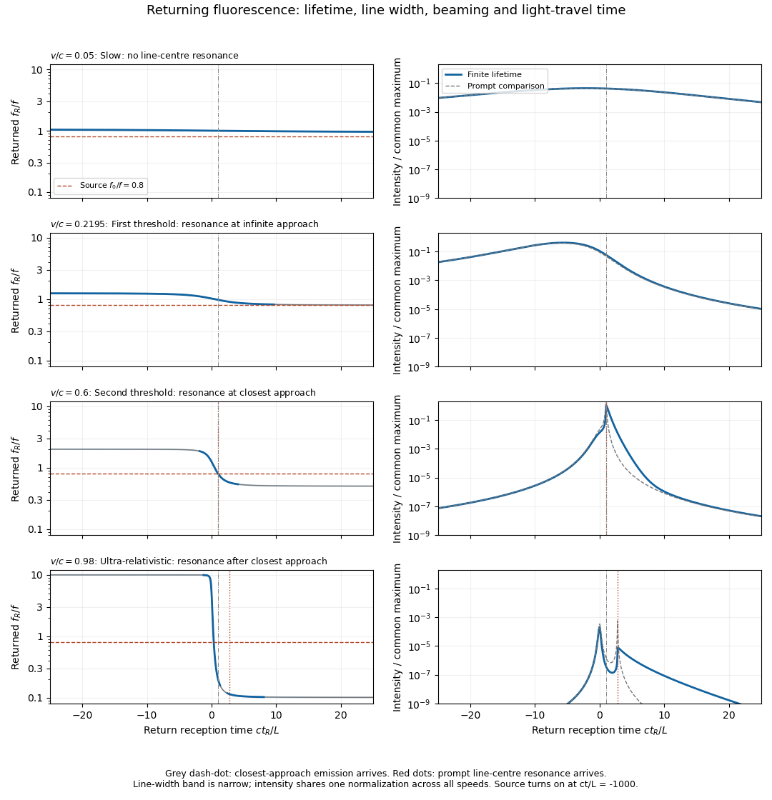
Illustrative returning fluorescence for slow motion, both resonance thresholds, and ultra-relativistic motion
. Left panels show the returned atomic line centre and its finite-width band; a dashed line marks the source frequency. Right panels show received intensity on a common logarithmic scale, with a thin curve for the zero-lifetime comparison. The model uses f0/f equal to 0.8, proper lifetime c tau/L equal to 0.4, fractional natural full width 0.02, and a finite source turn-on. Solid curves include the population decay, retarded reception and beaming. Details.
A model for fluorescence from a uniformly moving cloud generating the plotted envelopes iswhere is a Lorentz line shape of full width . The factor is the incident photon-flux correction per source-frame time. The population is an exponential memory of earlier absorption events, not an instantaneous resonance indicator. For a detector of fixed small area at the origin, its received bolometric intensity scales asTwo powers of come from aberration of light, one from photon energy, and one from arrival-rate compression. Finite lifetime is dilated to in the source frame; over an interval with slowly changing geometry its observed decay time is . Thus approach can compress and amplify a pulse, while recession stretches and redshifts it. Illumination and collection each supply an inverse-square geometric factor in the prompt weak-excitation limit. Strong forward beaming can even make a detuned approaching precursor brighter than the later line-centre feature, as in the ultra-relativistic row; the intensity maximum need not occur at exact resonance.
Absolute amplitude and a unique detailed spectral line profile cannot be inferred from alone: cloud size, atom number, source power, optical depth, angular emission pattern and saturation were not specified. Finite cloud size convolves these point-centroid curves with additional delays. The plots describe incoherent, frequency-redistributed emission near ; a coherent Rayleigh scattering component would instead retain the driving frequency in the atom frame and add a different spectral component. These qualifications do not change the kinematic resonance thresholds or return-time relations.
Past exam of the symmetry and relativity course of the University of Oxford 2019 1 f iii Solution 2026-10-25
Every event is in both the causal future and causal past, soDrawing just the nearest two null rays on a temporally identified strip would miss winding causal curves and give an incorrect nonempty exterior region.
Past exam of the symmetry and relativity course of the University of Oxford 2019 1 f ii Solution 2026-10-25
Choose an integer sufficiently negative that . That lift lies in the ordinary causal past of the origin, and its projected causal curve reaches the origin. HenceFuture-directed curves can connect the origin and an arbitrary event in either order. This property includes the origin's nontrivial closed timelike curves.
There are unlisted articles, also show them or only show them.