
Removing from the closed interval leaves the separation of a topological spaceThus is a cut point of .
In contrast, removing any point from the square leaves a path-connected space. To prove this, take distinct . Choose an interior point outside the two lines through and . Such a choice exists: a small circle in the interior meets each of those lines in at most two points. Since is a convex set, the line segments and stay in ; our choice of ensures that both avoid . Their concatenation is a continuous path from to in .
The product topology on agrees with its usual subspace topology in the Euclidean plane. If were a homeomorphism, its restriction would give a homeomorphismThe domain is connected, since path connectedness implies connectedness, while the target is not connected. This contradicts the preservation of connectedness by a homeomorphism.
Suppose were compact. By the compact subset of a Hausdorff space theorem, it would be closed in , hence closed in . The singleton is also closed in the Hausdorff space : each other point has an open neighbourhood avoiding .
Consequently both and are clopen in . They are disjoint, nonempty, and cover , giving a separation of a topological space in contradiction to the connectedness of . Thus is not compact.
The intended hypothesis is that is not connected. The original PDF has the same grammatical ambiguity as the transcription. If only were assumed not connected, the assertion would fail for the discrete space with its usual metric and the closed subset : two disjoint sets cannot both meet that singleton.
Under the intended reading, choose a separation of a topological space . Both and are nonempty and closed in , because each is the complement of the other relatively open part. Since is closed in , both are closed in .
For a nonempty subset of the metric space , the distance to a set satisfiesIndeed, the triangle inequality gives , and swapping proves the bound. Thus the two distance to a set functions below are continuous. SetThese are disjoint open sets. For , we have and , since is closed and . Hence . Similarly . Therefore and both and meet , as required. The construction is a concrete instance of the normality of every metric space.
Use the Sierpiński space with topology . The singleton is compact: from any open cover, choose one member containing . But is not open, so is not closed. This also exhibits why the Hausdorff hypothesis in the preceding proof matters.
Let be compact, with a Hausdorff space. The empty set is closed, so suppose . Fix . For each , the Hausdorff property supplies disjoint open neighbourhoods of and of .
The form an open cover of . Choose a finite subcover and put . This is an open neighbourhood of . If a point of belonged to , it would belong to some as well as , a contradiction. Hence . Every point of the complement has such an open neighbourhood, so is open and is closed.
Let be an open cover of by open subsets of . The continuity of makes each preimage open in , and these preimages cover . By compactness, choose withApplying gives . Thus every open cover of has a finite subcover, proving the continuous image of a compact space theorem. A cover by sets open in gives the same argument after expressing them as intersections with ambient open sets.
Give the nonempty subset its subspace topology. It is compact if every open cover admits a finite subcover. Equivalently, whenever with each open in , there are such that .
It is connected if it has no separation of a topological space: there are no disjoint nonempty open subsets of with . Here openness is relative to the subspace topology; equivalently, the only clopen sets of are and .
Every complete polygon edge pairing gives a compact connected surface with empty manifold boundary. Here is the local reason at the vertices. Replace each polygon corner by a small link interval. The polygon edge pairings identify all endpoints of these link intervals in pairs. In a given vertex equivalence class, the resulting graph is connected: the endpoint identifications generating that vertex equivalence class also connect its corner intervals. Every link graph vertex has degree of a vertex two, so the graph is a circle. Its topological cone is a disc, giving the required local surface model. Edge and face CW cell interiors have the usual disc neighbourhoods as well. A finite triangulation compatible with the polygon edge pairings realizes the result as a finite simplicial complex, giving a Hausdorff, second-countable space.
For every such surface, . If it is orientable, the classification of compact surfaces gives , so or . If it is a nonorientable surface, write for its nonorientable genus; then gives . The exhaustive list is therefore
- the sphere ;
- the torus ;
- the real projective plane ;
- the Klein bottle ;
- the connected sum of surfaces , a nonorientable surface of nonorientable genus three.
To prove that every listed possibility actually occurs, the following six-letter boundary words specify complete pairings of a hexagon:The vertex counts follow by matching starts and ends of equally directed arrows, just as in part (b). The first and third words pair every letter with its inverse, giving orientable surfaces. Each other word contains a letter twice with the same sign, giving a nonorientable surface: an orientation on the face would induce equal, rather than opposite, boundary directions along that glued pair. With the displayed Euler characteristics, the classification of compact surfaces identifies the examples exactly as listed. All five types occur, and no others occur.
A complete pairing of the six polygon edges leaves three edges and one face as CW cells, together with the vertex equivalence classes. If denotes their number, then and the polygonal-schema Euler count givesA closed orientable surface of genus two has Euler characteristic . Since the Euler characteristic is a topological invariant, no complete pairing of a hexagon can give that surface. Equivalently, the polygonal-schema Euler count bounds the genus of an orientable result by , so .
False: the result is again a torus with one open disc removed. Label the hexagon polygon vertices clockwise from the upper left asWith the same arrow labels as in part (ii),There are two vertex equivalence classes, and . The free diagonal polygon edges are and . Each joins to , so together they form one boundary component of a surface, not two. At each vertex equivalence class the three corner sectors join in a single chain between these two free polygon edges. Thus each vertex link in a polygonal schema is a closed interval, and the quotient space is an orientable surface with boundary.
Its CW complex has CW cells comprising two vertices, four edges and one face, givingIn contrast, a torus with two disjoint open discs removed has two boundary components of a surface and Euler characteristic . Either topological invariant rules out the proposed homeomorphism.
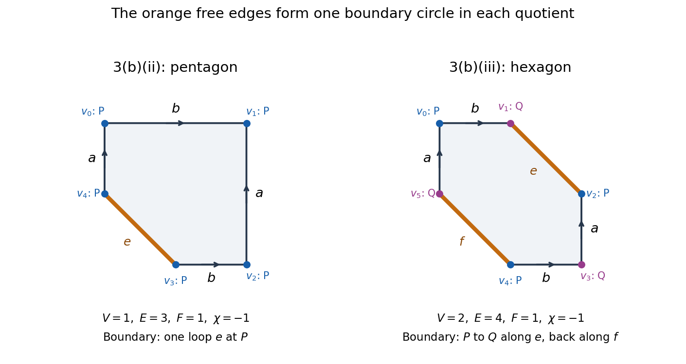

True. Label the pentagon polygon vertices clockwise from the upper left asUse for the upward single arrows and for the rightward double arrows in the original diagram. Their endpoint identifications areAll five polygon vertices are therefore identified. The remaining diagonal polygon edge, from to , has its endpoints identified and is the only boundary component of a surface.
The paired polygon edges join half-disc neighbourhoods into disc neighbourhoods. At the common vertex, the five corner sectors join in one chain whose two free ends lie on the unpaired polygon edge: its vertex link in a polygonal schema is a closed interval. Hence that point has a half-disc neighbourhood. This verifies that the quotient space is a surface with boundary, rather than merely counting its CW cells. The paired polygon edges are oppositely traversed around the polygon, so this surface is orientable.
Label the hexagon polygon vertices in the direction in which its boundary word is , with the first side running from to . Matching the endpoints according to the arrows givesThus the two vertex equivalence classes are and .
The polygonal schema gives a compact connected surface with empty manifold boundary. Interior points have disc neighbourhoods; a paired polygon edge glues two half-disc neighbourhoods into a disc. At each of the two vertex equivalence classes, its three corner sectors join cyclically, so the vertex link in a polygonal schema is a circle, again giving a disc neighbourhood. Pairing every label once positively and once negatively makes these gluings consistent with an orientation, so the resulting surface is orientable.
The resulting CW complex has CW cells comprising two vertices, three edges and one face. Its Euler characteristic isBy the classification of compact surfaces, a connected closed orientable surface with has genus satisfying , hence . The quotient space is a torus.
Let be the common point of the two circles. For sufficiently small , the open neighbourhoodhas the following local structure: consists of four disjoint open arcs, an upper and a lower branch from each circle. These are its four connected components, each open and closed relative to .
Suppose a coordinate chart of some dimension of a manifold existed at . The case would make an isolated point, which it is not. For , shrink the chart inside so that its image is an open ball centred at the image of . Its domain of a function is an open neighbourhood of , so it meets all four arms of . Intersecting those arms with gives four disjoint nonempty clopen sets partitioning ; hence there are at least four connected components.
But a punctured ball in has exactly two connected components, and a punctured ball in for is path-connected. A homeomorphism preserves connected components, giving a contradiction in every dimension of a manifold. Thus is not a topological manifold. The argument uses arbitrarily small coordinate charts; the fact that the whole has two pieces alone would not be a local obstruction.
The unit circle is Hausdorff and second countable, since both properties pass to topological subspaces of the Euclidean plane. To exhibit its local coordinate charts, consider the four open semicirclesThey cover . On , the projection map is a homeomorphism onto the open interval , with continuous inverse functionOn , use , with inverse function . These coordinate charts show that is a one-dimensional topological manifold with empty manifold boundary.
Let , and choose in each circle the point opposite :In the subspace topology from the Euclidean plane, the sequence converges to , which does not belong to . Thus is not closed in .
On the other hand, let . With the quotient map from part (i),This is closed in : its complement is the open set . The definition of the quotient topology, applied to complements, says that is closed in . A homeomorphism would carry this closed set to the closed set , a contradiction. Therefore is not a homeomorphism.
The obstruction occurs at the common point. The open set contains the collapsed point, but its image contains no neighbourhood of , since . The wedge sum topology allows a separate small neighbourhood on each circle; a neighbourhood of in the Hawaiian earring must contain all sufficiently small whole circles.
Use positive indices and write . SetFor fixed , this function is a homeomorphism from the unit circle to : it scales its radius to and translates its centre to . Thus it takes values in the Hawaiian earring and is surjective onto . It is continuous on each open slice ; since these slices form an open cover of , is continuous on the whole product topology.
Distinct circles meet only at . To see this directly, their equations areFor , subtraction gives , then . Each slice contains exactly one preimage of , namely . Therefore the only nonsingleton fibre of is .
Let be the quotient map collapsing . The universal property of the quotient topology supplies a unique continuous map with . The fibre calculation proves injectivity, and surjectivity follows from that of . Hence is the required continuous bijection.
False, with “disjoint union” understood as a topological disjoint union. Take the rational numbers with the usual subspace topology from the real line.
Every connected subset of has at most one point. Indeed, if it contained , choose an irrational number . The two relatively open setspartition and separate any subset containing both and . Hence the connected components of are singletons.
If a topological disjoint union of nonempty connected spaces were homeomorphic to , the image of each summand would be connected, hence a singleton. Every summand would therefore be a one-point topological space. Their topological disjoint union is a discrete space, since each summand is open. But is not a discrete space: for each , the distinct rational numbers approach , so is not an isolated point. This is a contradiction. The set decomposition into connected components always exists; giving those pieces the topological disjoint union topology need not recover the original topology.
The sphere is path-connected. For which are not an antipodal pair, a continuous path isThe denominator never vanishes: a zero would make and antipodal. If , choose a unit vector perpendicular to and concatenate the paths from to and from to of the same form. Thus is connected. The quotient map is continuous and surjective, so the continuous image of a connected space theorem proves that is connected. In fact composing the paths above with also proves path connectedness.
Let and be the quotient maps. The continuous mapis a homeomorphism onto the upper hemisphere; its inverse function is the restriction of the projection map . Every antipodal pair on meets that hemisphere. Moreover, two points of this hemisphere are antipodal only if both lie on the equator. ThusBy the universal property of the quotient topology, induces a continuous bijection
To justify continuity of the inverse function, the source is compact, being a continuous image of a compact space ; the Heine-Borel theorem gives compactness of . The target is Hausdorff, as follows. For distinct equivalence classes , putIn , take the union of the two relative open balls of radius about , and similarly take about . Every distance between their respective centres is at least , so the triangle inequality gives . These open sets contain entire antipodal pairs, hence and similarly for . The quotient topology therefore makes and disjoint open neighbourhoods of the two classes.
For the sphere model of the real projective plane, letThen with the quotient topology: each equivalence class is an antipodal pair.
For the closed disc model, letGive the quotient topology. Only antipodal pairs on the boundary circle are identified in the closed disc model; interior points remain distinct.
There are unlisted articles, also show them or only show them.