
Past exam of the topology and groups course of the University of Oxford 2023 1 b ii Solution 2026-10-25
DefineThe two formulas agree on the attached end, so the universal property of the quotient topology makes a continuous map. Also .
Slide each cylinder point towards its attached end usingAt these formulas both give , so they define a homotopy on the mapping cylinder. For continuity, the product of a quotient map with the unit interval is a quotient map; the formulas before taking the quotient topology are continuous maps and agree on every identified pair. ThusMoreover stays fixed throughout. We have obtained the stronger conclusionIn particular is the requested homotopy retract.
Past exam of the topology and groups course of the University of Oxford 2023 1 b i Solution 2026-10-25
Writefor the quotient map defining the mapping cylinder, and put . Since the equivalence relation only attaches points at height to , distinct points at height remain distinct. Thus is an injective continuous map.
Define the homotopyIt is a continuous map, with and . HenceEven if identifies many points, the free end of the mapping cylinder retains a separate copy of every point of .
Past exam of the topology and groups course of the University of Oxford 2023 1 a iii Solution 2026-10-25
Let be the inclusion map and the retraction. Since is contractible, choose a contraction of a topological spaceThe function compositionis a continuous map. Its endpoints satisfyConsequently is a homotopy from the identity map of to a constant function. This provesThe contracting point of need not belong to : applying the retraction sends it to the contracting point of . This is the retract of a contractible space principle.
Past exam of the topology and groups course of the University of Oxford 2023 1 a ii Solution 2026-10-25
Yes. Take , the circle, and . The constant function is a continuous map and satisfies , so is a retract of .
However, their fundamental groups areA homotopy equivalence between path-connected spaces induces a group isomorphism of their fundamental groups, allowing the usual change of base point. The infinite cyclic group is not the trivial group. Therefore a retract need not have the homotopy type of its ambient space.
Past exam of the topology and groups course of the University of Oxford 2023 1 a i Solution 2026-10-25
Two continuous maps are homotopic if there is a continuous mapHere the Cartesian product has the product topology. Such an is a homotopy, written .
The topological spaces are homotopy equivalent if there are continuous maps and such thatEach is then a homotopy inverse of the other.
For with its subspace topology with inclusion map , a homotopy retract, in the course's convention, is a continuous map withThus is an actual retraction, and give a homotopy equivalence. Requiring the latter homotopy to fix pointwise at all times gives the stronger condition of a deformation retraction as used in this wiki. The course's definition of homotopy retract requires no such restriction on that homotopy.
Past exam of the topics in fluid mechanics course of the University of Oxford 2023 3 c iii Solution 2026-10-25
For the approximate similarity profile, , and thereforeFor the prescribed undisturbed horizontal streams, a suitable choice is , which gives zero transverse velocity at both far-field limits. Then inside the layer. The nonzero internal crossflow is consistent with the streamwise widening of the velocity transition.
Another possible convention is to make the line a streamline, imposing . This requires , equivalently , and gives . It therefore requires a uniform outer crossflow relative to the coordinates used for the centred error function profile. A single constant cannot impose both zero far-field crossflow and unless . The physical lateral boundary conditions, or the chosen material centreline, determine which convention is appropriate. Since , these transverse velocities are of order for fixed .
Past exam of the topics in fluid mechanics course of the University of Oxford 2023 3 c ii Solution 2026-10-25
The two external stream velocities imposeLet and seek over . The nonlinear term is then , so the leading ordinary differential equation isFor , this is the first-order linear differential equation . Its integrating factor is , giving . An integration using the error function givesThe two far-field boundary conditions require and . A second integration usesConsequentlyThe relation between and cancels the extra term when differentiating. It gives the familiar error function mean velocity profileto first order in . The additive constant does not affect this velocity profile at the retained order; its interpretation comes from the transverse velocity.
Past exam of the topics in fluid mechanics course of the University of Oxford 2023 3 c i Solution 2026-10-25
Assume and set . With independent of , balancing streamwise transport with transverse mixing gives a layer width proportional to . Write its constant slope asHere is a spreading constant associated with the chosen definition of thickness; it is unrelated to the capillary in Question 1. The origin selects zero virtual-origin offset.
Define , , and introduce the stream functionThis automatically satisfies incompressibility and yieldsFor the momentum equation, use and :Because , the common coefficient cancels, giving the turbulent mixing-layer similarity equationThe boundary layer approximation also requires , consistently with the assumed slow spreading.
Past exam of the topics in fluid mechanics course of the University of Oxford 2023 3 a iii Solution 2026-10-25
The product rule and fluctuation incompressibility give the pointwise identityAveraging therefore givesThe fluctuation term is consequently the divergence of a Reynolds stress. The eddy viscosity model represents this momentum transport through a coefficient multiplying the mean strain-rate tensor:for its shear or deviatoric part. For example, in a thin parallel shear flow. The dynamic viscosity is an effective flow-dependent transport coefficient, rather than a molecular material property. Large eddies carry linear momentum between regions of different mean velocity.
There is a necessary qualification to the printed tensor equation (4). Taking its trace literally gives , which would exclude nonzero turbulence. A consistent deviatoric eddy-viscosity closure in fluctuating dimensions isThe isotropic term is absorbed into the effective pressure . Here for a strictly two-dimensional fluctuation model. The subsequent equations use for this effective pressure, or equivalently use (4) as a shear-stress closure. This preserves the intended thin-layer model without asserting an impossible full covariance identity.
For turbulent motions of scale and velocity scale , the estimate gives . It is much greater than one on energetic large scales and in the inertial range well above the Kolmogorov length scale. At the molecular dissipation scales it is no longer large, and molecular transport also dominates very near a smooth solid wall.
Past exam of the topics in fluid mechanics course of the University of Oxford 2023 3 a ii Solution 2026-10-25
Write and , with . Assume a statistically stationary mean and sufficient regularity for Reynolds averaging to commute with spatial derivatives. Thenprovided the endpoint difference grows sublinearly. Averaging the continuity equation givesIn Einstein notation, the nonlinear term expands asThus the Reynolds-averaged Navier-Stokes equation isThe extra term survives because the average of a product of zero-mean fluctuations need not vanish; it represents turbulent transport of mean linear momentum.
Past exam of the topics in fluid mechanics course of the University of Oxford 2023 3 a i Solution 2026-10-25
For a constant-mass density incompressible flow with no imposed body force, the two-dimensional Navier-Stokes equation isA conservative body force, if retained, may be incorporated into a modified pressure. Using scales and givesHere is the molecular kinematic viscosity. At high Reynolds number, inertia and the pressure gradient dominate on the outer length scale, while molecular viscous diffusion is small there. Thin boundary layers, narrow shear flows and fine turbulent scales can still have sufficiently large velocity gradients for viscous effects to matter. High Reynolds number permits instability and turbulence, but does not alone prove that every flow is turbulent. Molecular viscous dissipation remains essential at the small end of the turbulent cascade.
Past exam of the topics in fluid mechanics course of the University of Oxford 2023 2 c iii Solution 2026-10-25
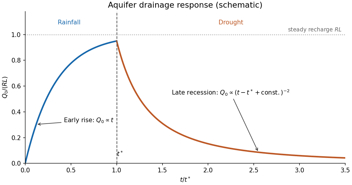
Let . The spatial ordinary differential equation gives , so its leading outlet behavior isAgain this is a square-root drainage boundary. For the separable aquifer drawdown, the dimensional drainage flux isEquivalently, with , it is for an exact separated profile. Integrating the spatial ordinary differential equation gives . This verifies the global mass conservation checkThus the late drainage flux follows an inverse-square power law, while stored water decays inversely with time.
The aquifer drainage hydrograph starts at zero, rises linearly in the early rainfall similarity solution, and approaches the total recharge if rainfall lasts long enough for a finite-length steady state. Indeed, steady mass conservation gives and , hence . At , the outlet flux stays continuous for a regular inherited flux profile, then recedes as water drains; the eventual decay is proportional to . An arbitrary transition requires the full time-dependent partial differential equation, so matching an early rainfall formula directly to a separated drought formula is only a schematic approximation.

Past exam of the topics in fluid mechanics course of the University of Oxford 2023 2 c ii Solution 2026-10-25
With , substitute into the dimensional Boussinesq equation for an unconfined aquifer:For a positive draining profile, take . Normalize , so has the dimensions of height. The temporal ordinary differential equation integrates toThe spatial ordinary differential equation and boundary conditions areHere has units of inverse length with this normalization. The scale freedom between and is fixed by the chosen value ; the amplitude of , and hence , must be matched to the available water.
This separable aquifer drawdown is exact if the inherited height profile has the separated spatial shape. For a general rainfall-generated initial condition, it describes the late drought regime; it cannot reproduce an arbitrary profile at the instant rainfall stops merely by choosing one temporal constant.
Past exam of the topics in fluid mechanics course of the University of Oxford 2023 2 c i Solution 2026-10-25
Return to dimensional variables. The river at base level imposes the drained boundary condition, while the right-hand end is impermeable:As long as the right-hand end remains wet, the latter is . The initial condition for the drought is the height profile inherited at ; stopping rainfall changes the forcing but does not instantaneously remove stored water.
Past exam of the topics in fluid mechanics course of the University of Oxford 2023 2 b iii Solution 2026-10-25
Introduce the positive outlet constantFor a draining similarity profile, is finite and positive. A regular linear profile would have and at the origin, incompatible with the rain-fed aquifer similarity solution . Instead there is a square-root drainage boundary. At leading order, , givingMore explicitly, the rain-fed aquifer similarity solution implies , hence and . The height vanishes but its derivative diverges; their product remains finite.
Use temporarily for dimensional quantities. The nondimensionalization in part (a) givesTaking the drainage flux to be positive out of the left-hand end, , givesThe printed expression in terms of and must be understood as this limit; a literal product of their separate endpoint values is undefined. This is discharge per unit transverse width. Very close to the river, the divergent slope marks the limit of the Dupuit approximation, while the outer solution still supplies the leading discharge.
Past exam of the topics in fluid mechanics course of the University of Oxford 2023 2 b ii Solution 2026-10-25
The condition means the river maintains the water table at the impermeable base level: . The liquid is exposed to atmospheric pressure there. It does not imply zero drainage, because may be singular at the outlet.
Far from the river, lateral drainage has not significantly affected storage. Rainfall simply fills pore volume, so the dimensional height is . In the dimensionless variables this is , giving .
Although the physical aquifer is finite, these boundary conditions describe its early similarity solution before the drainage-affected region reaches . In dimensional variables its horizontal extent is of order , so the semi-infinite approximation requires .
Past exam of the topics in fluid mechanics course of the University of Oxford 2023 2 b i Solution 2026-10-25
Use the dimensionless equation from part (a). For the similarity ansatz , , its three terms have time factorsA nontrivial similarity solution retaining storage, lateral drainage and nonzero rainfall requires the exponents to agree:Unlike a source-free diffusion equation, the nonzero prescribed rainfall fixes an amplitude-versus-time scale directly, so no additional conserved quantity or boundary condition is required to determine these exponents. Degenerate spatially uniform solutions are an exception to this all-terms balance. The rain-fed aquifer similarity solution satisfiesIf the dimensional equation is used directly without scaling out coefficients, its similarity profile instead obeys . The normalization above is the one in which the subsequent condition applies.
Past exam of the topics in fluid mechanics course of the University of Oxford 2023 2 a iv Solution 2026-10-25
Set , , and . The Boussinesq equation for an unconfined aquifer becomesBalance rainfall recharge with lateral drainage, and then with storage:Dropping tildes, the dimensionless equation isThe horizontal Darcy velocity, vertical Darcy velocity, and discharge scales are respectively , , and . Thus the vertical thickness scale is set by rainfall balanced against hydraulic conductivity over the finite drainage length , rather than by porosity. The latter determines the storage time . The Dupuit approximation requires for these scales. The initially dry initial condition is .
Past exam of the topics in fluid mechanics course of the University of Oxford 2023 2 a iii Solution 2026-10-25
The hydrostatic pressure gives , independent of depth. Thus Darcy's law gives and the horizontal volume flux per unit width isThe coefficient is the hydraulic conductivity, with units of velocity. For a column of unit horizontal area, the stored water volume is , and rainfall supplies volume flux . The local mass conservation equation is . Therefore the Boussinesq equation for an unconfined aquifer isThis assumes rainfall is entirely converted into recharge and neglects unsaturated storage and losses before the water reaches the water table.
Past exam of the topics in fluid mechanics course of the University of Oxford 2023 2 a ii Solution 2026-10-25
Let be the characteristic saturated thickness and let . Scale pressure by . The horizontal part of Darcy's law gives the scaleBy incompressibility, . The vertical part of Darcy's law isIts left side is smaller than the scale by . Therefore , and the leading pressure is hydrostatic pressure:Here the water table has pressure . This is the Dupuit approximation, valid away from the small region near an outlet where the surface slope need not remain small.
There are unlisted articles, also show them or only show them.