
Past exam of the symmetry and relativity course of the University of Oxford 2019 1 f i Solution 2026-10-25
For any representative event , choose an integer large enough that . A future-directed timelike segment from the origin to that lift projects to a causal curve on the quotient. ThereforeEven points with large can be reached by allowing sufficiently many temporal windings. The purple lower-right panel in part c denotes simultaneous membership in both the causal future and causal past.
Past exam of the symmetry and relativity course of the University of Oxford 2019 1 e iii Solution 2026-10-25
The complement of the causal future and causal past isThis green region is confined to and meets the identified strip edges. Spatial periodicity creates alternative signal paths, but time remains noncompact and no closed timelike curve follows from this spatial identification.
Past exam of the symmetry and relativity course of the University of Oxford 2019 1 e ii Solution 2026-10-25
The causal past follows from the same covering-space argument with reversed endpoints:For , the whole spatial circle can send a causal signal to the origin. The lower-left spacetime diagram in part c is therefore completely orange sufficiently far below the origin.
Past exam of the symmetry and relativity course of the University of Oxford 2019 1 e i Solution 2026-10-25
A causal curve can wind around the spatial circle. Lift its endpoint to on the covering space. A lift is reachable from the origin if for at least one integer . With shortest circular distancethe causal future isIn the centred fundamental strip, . For , every spatial point is in the causal future. This produces the fully blue upper part of the lower-left panel in part c.
Past exam of the symmetry and relativity course of the University of Oxford 2019 1 d iii Solution 2026-10-25
The invariant spacelike condition is . Hence the primed-coordinate events in neither the causal future nor the causal past obeyThe green regions in part c retain their shape in primed coordinates. A particular spacelike event's coordinate time may change sign, but it never enters either light cone.
Past exam of the symmetry and relativity course of the University of Oxford 2019 1 d ii Solution 2026-10-25
The same Lorentz transformation maps the past light cone to itself. In the primed axes the causal past isthe orange region in the upper-right spacetime diagram of part c. Future and past are not interchanged by the standard boost.
Past exam of the symmetry and relativity course of the University of Oxford 2019 1 d i Solution 2026-10-25
For the standard passive Lorentz boost, write andA proper orthochronous Lorentz transformation preserves the sign of the time component of a nonzero future causal vector and preserves its Minkowski norm. ThereforeThe upper-right panel of part c uses horizontally and vertically. Its null rays still have slopes . The grey dashed old axes satisfy for the old time axis and for the old spatial axis; changing the coordinate grid has not changed which events are reachable.
Past exam of the symmetry and relativity course of the University of Oxford 2019 1 c iii Solution 2026-10-25
Outside both light cones, the separation from the origin is spacelike. Thus the events in neither the causal past nor the causal future areNo causal curve can connect either endpoint to the other. These are the two green side regions in part c; the strict inequality excludes the causally reachable null boundaries.
Past exam of the symmetry and relativity course of the University of Oxford 2019 1 c ii Solution 2026-10-25
Reverse the endpoints of the future-directed causal curve. The origin can be reached precisely from its causal past,This is the orange region below the two null rays in part c. The origin itself belongs to both the causal future and causal past by the usual zero-length-curve convention.
Past exam of the symmetry and relativity course of the University of Oxford 2019 1 c i Solution 2026-10-25
A future-directed causal curve from the origin has . Integrating this inequality gives the causal futureThe straight timelike or null segment proves sufficiency. This is the blue region above the two null rays in the upper-left spacetime diagram of part c.
Past exam of the symmetry and relativity course of the University of Oxford 2017 3 b b Solution 2026-10-25
For , the laboratory wavevector is perpendicular to the boost. The dot product vanishes, soThis transverse-observer transformation is a blueshift. It must not be confused with the inverse factor often quoted when transverse refers to a ray perpendicular to the source velocity in the receiver's frame. The angle condition is specified in different frames in those two statements; relativistic aberration relates them.
Past exam of the symmetry and relativity course of the University of Oxford 2017 2 d b Solution 2026-10-25
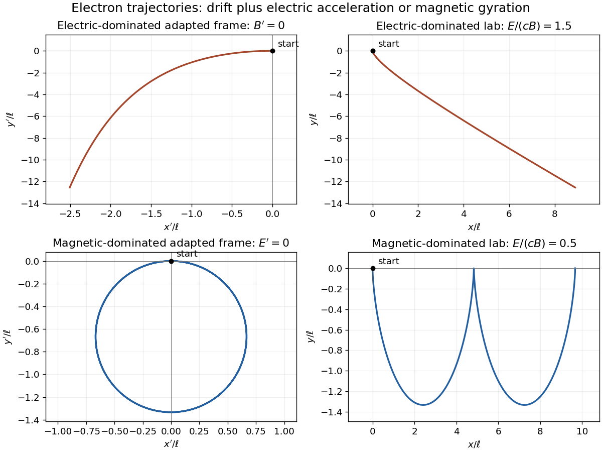
For the magnetic-dominated crossed-field orbit, choose along , which is subluminal when . Then and . The initial velocity in this frame is , and the constant particle Lorentz factor is because a magnetic field does no work.
Define the signed relativistic cyclotron frequency , retaining . With as parameter, the exact primed trajectory isIt is a circle of radius with centre ; its initial velocity is as required. Transforming back givesIn the laboratory this is a stretched cycloidal trajectory with cusps where the electron is instantaneously at rest. Its average drift is , along for the positive field orientation. Its energy oscillates as the electric field exchanges energy with it; it does not accelerate without bound. If , the initially stationary electron remains stationary. At , neither of these finite boosts exists; that separate null-field limit is not one of the two strict cases requested.

Past exam of the symmetry and relativity course of the University of Oxford 2017 2 d a Solution 2026-10-25
For the electric-dominated crossed-field orbit, choose a boost along . Since , it is subluminal. The Lorentz transformation of electromagnetic fields gives and , where . The initially stationary electron has , not zero velocity in this frame.
Let , and . Neglect radiation reaction, as in the prescribed external-field model. Integrating the relativistic Lorentz force in this purely electric frame gives the exact trajectoryIndeed , , and satisfy both the force equation and . The constant transverse momentum must be retained.
The inverse boost gives a useful exact laboratory parametrization as well:For , the lab electron starts accelerating toward negative and bends toward positive , the direction of . It never acquires a cyclotron orbit in this electric-dominated case. At late times, and , so its speed approaches along an oblique asymptote. Reversing field signs reverses the appropriate directions. The zero- limit is the ordinary electric-field hyperbolic motion.
Past exam of the symmetry and relativity course of the University of Oxford 2017 2 c b Solution 2026-10-25
Past exam of the symmetry and relativity course of the University of Oxford 2017 2 c a Solution 2026-10-25
Put . The total four-momentum of the perpendicular photons isAlthough each constituent is massless, the sum has . Its invariant mass is thereforeThe rest energy is the total energy in the frame where the two photon momenta cancel, not the sum of individual photon rest energies.
Past exam of the symmetry and relativity course of the University of Oxford 2016 4 d iii Solution 2026-10-25
The final unnumbered force question has this inferred third subpart. For either wire's exterior field,This electromagnetic field invariants is positive in every inertial frame. A purely magnetic nonzero field would instead have . Thus no physical boost makes the interaction purely magnetic. There is a comoving frame with a purely electric interaction, which is consistent with the invariant's sign.
The convected charge current gives the same conclusion. Its effective line-current invariant is , so no inertial frame can neutralize the charge while leaving only a current. In particular for a longitudinal boost of speed , cannot vanish when .
For two identical wires separated by , the laboratory transverse force per unit length isElectric repulsion exceeds the magnetic attraction. This assumes each moving wire has uncompensated convected charge; a neutral wire carrying conduction current is a different charge-current system and has a different invariant classification.
Past exam of the symmetry and relativity course of the University of Oxford 2016 4 d ii Solution 2026-10-25
Boost the comoving electric field perpendicular to itself along the wire. The transverse electric field gains a factor , while a circulating magnetic field appears. Equivalently apply Gauss's law and Ampère's law with laboratory line charge and current :These are exterior fields of the ideal straight wire. For laboratory line density , substitute ; for proper line density , substitute . The radial distance is transverse to the boost and unchanged between the two frames.
Past exam of the symmetry and relativity course of the University of Oxford 2016 4 d i Solution 2026-10-25
Model the wire as an infinite straight line along . Let be its rest-frame line charge density and its laboratory line charge density. Length contraction gives . If the symbol in the source is intended as volume charge density, replace these line densities by their integrals over the cross section; an unspecified wire radius does not determine an interior field.
In the comoving frame the wire is static, so Gauss's law and cylindrical symmetry give the exterior fieldsIf the source's means laboratory line density, this electric field is ; if it means proper line density, it is . Stating the density's reference frame is necessary for an unambiguous factor of .
Past exam of the symmetry and relativity course of the University of Oxford 2016 4 c b Solution 2026-10-25
In a transparent uniform medium, constructive phase interference along the trajectory requires . Since , the Cherenkov cone angle obeysHere , so emission is allowed andThe electron is not an isolated vacuum particle: it interacts with the dielectric polarization of the medium. Here the angle describes the photon direction relative to the trajectory; the conical wavefront surface has the complementary angle.
This angle is the classical or negligible-recoil result. At finite photon energy, energy-momentum bookkeeping in a nondispersive medium gives a recoil correction proportional to ; no photon frequency is supplied for such a correction. In a dispersive medium use separately for each transparent frequency band.
There are unlisted articles, also show them or only show them.