
Set . The equilibrium equations cancel the constant gravitational and elastic terms, leaving the small-oscillation mass and stiffness matricesThe off-diagonal mass terms arise because rope-length coordinates are not absolute climber displacements. For any nonzero velocity vector, , so is a positive-definite matrix.
Within the vertical Hookean model, the displacement equations are exactly linear while all ropes stay taut. Small amplitudes ensure that none reaches the slack regime .
Past exam of the mathematics course of the year 2 of the natural sciences course of the University of Cambridge 2015 Paper 2 7 b Solution Created 2026-10-18 Updated 2026-11-05
The Euler-Lagrange equations giveFor example, differentiating with respect to collects contributions from all three climbers, because changing moves all of them. At equilibrium, all accelerations vanish, soThe top rope supports the total weight, while each lower rope supports only its own climber. These extensions are positive, consistent with the taut-rope tension law.
Take downward vertical distances from the support. The climber positions are , and . Their kinetic energy is thereforeIntegrating the tension-extension relation gives the elastic potential energy for each taut rope. Because downward displacement lowers gravitational potential,An arbitrary additive constant in is immaterial. This is the vertical-motion model implicit in using only rope lengths as generalized coordinates; swinging angles are not additional degrees of freedom in this model.
The scalar, symmetric-traceless and axial tensor decomposition fixes the scalar part by the trace:Subtracting this isotropic part from the symmetric tensor in part (c) givesIts trace is zero. The antisymmetric tensor part isAdding reconstructs every entry of .
Subtracting a scalar multiple of the identity preserves every eigenvector: if , then . Thus the principal axes are the same as in part (c), with shifted principal valuesThe two tensors are coaxial symmetric tensors. At both vanish, so neither specifies unique axes.
Let . Averaging each pair of transposed entries gives the symmetric tensorFor , the upper block is the outer product of with itself. It sends that vector to times itself and annihilates its perpendicular. Thus its orthonormal principal axes and corresponding eigenvalues areTaking these vectors as the rows of the change-of-components matrix givesThis matrix is orthogonal with determinant one. These are the principal axes of a planar rank-one tensor block.
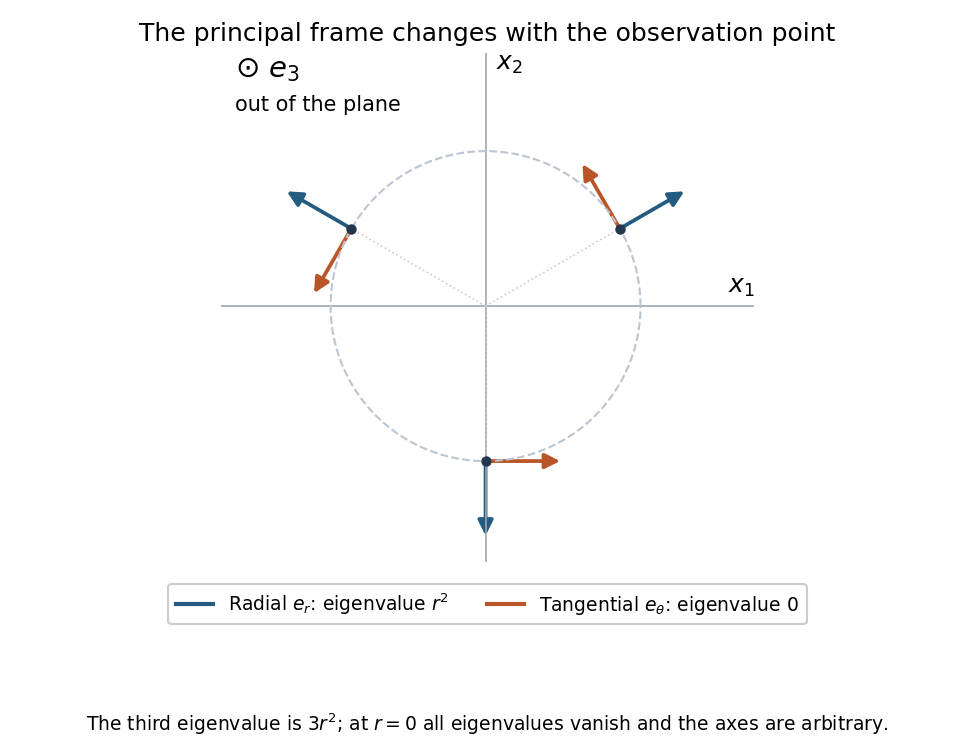
The radial and tangential principal directions rotate with position; the third principal axis is perpendicular to this plane
. Details. 
The matrix is a pointwise frame transformation: because its angle varies with position, it does not represent one fixed Cartesian rotation diagonalizing the entire field everywhere. On the axis , the symmetric tensor is zero; all principal values coincide and any orthonormal axes may be chosen. The displayed formula for is therefore used only off that axis.
Define the symmetric tensor and antisymmetric tensor parts by and . The transformed transpose satisfies . Thereforeand similarlyBoth obey the tensor component transformation law. Thus the symmetric and antisymmetric parts are themselves second-order tensors. Taking a transpose and forming linear combinations commute with this orthogonal change of frame.
Preserving Cartesian lengths and Euclidean inner products requires an orthogonal matrix:Its determinant is . Relative to an originally right-handed frame, gives a right-handed frame and a left-handed frame. More generally, this sign determines whether the two frames have the same or opposite orientation.
The tensor component transformation law isFor a tensor field, the components are compared at the same physical point, whose coordinates satisfy .
Use the Fourier transform convention . For a transformable response with the necessary boundary terms vanishing, integration by parts givesTransforming the differential equation therefore gives , soThe identities also hold for tempered distributions. The denominator factors as ; its two poles are in the upper half-plane, corresponding under inverse factor to the causal Green function of a damped oscillator.
The frequency-domain formula selects the Fourier-transformable response. Decay of the force alone would not remove arbitrary homogeneous solutions, which grow towards negative time and do not have an ordinary bilateral Fourier transform.
Choose a branch of the complex logarithm with , placing its branch cut down the negative imaginary axis. Thus for , while on the negative real axis for .
Integrate around an upper semicircle, with a small clockwise semicircular indentation above zero. The large arc contributes , and the small arc contributes . The only enclosed pole is , withWriting for the required integral, the negative real segment contributes . Hence the residue theorem givesThe imaginary terms cancel, leavingThe integral converges at both endpoints because is integrable near zero and is integrable at infinity. As a real-variable check, scaling reduces the result to the vanishing first logarithmic moment at , one of the logarithmic moments of the Cauchy kernel.
On the axis, the Poisson kernel for the upper half-space depends only on the radial boundary coordinate. Integrating over the disk givesTherefore the axial Poisson extension of a circular boundary patch isIt tends to one as the axis approaches the boundary inside the patch, and tends to zero as far above it.
The boundary values jump at the circular rim. They are understood almost everywhere, or as limits at continuity points; changing the assigned value on that measure-zero circle does not change the integral. At a rim point the vertical limit is one-half, rather than a continuous extension with the specified value on both sides of the jump.
Let the evaluation point be , , and reflect it to . The method of images constructsThe two Euclidean distances coincide on the plane, so there. The negative image source lies outside the domain; inside, only the real source contributes to . The difference also decays at infinity.
On the plane write and set . The outward unit normal of the upper half-space is . Direct differentiation givesSubstituting into the boundary representation from part (c) yields the Poisson kernel for the upper half-space:Its sign is positive, as expected from the maximum principle for nonnegative boundary data. Its normalization can be checked in polar coordinates:As the kernel is an approximate identity, recovering at its continuity points. Boundary data must have the decay and regularity compatible with the stated condition at infinity.
Impose the homogeneous Dirichlet boundary condition on the boundary variable:This removes the term containing the unknown normal derivative of . The prescribed boundary values alone then determine the solution throughFor an unbounded domain one also imposes the appropriate decay condition at infinity. This defines the required Dirichlet Green function.
Fix inside and put in Green's second identity. The volume integral becomesHere Laplace's equation eliminates the second term, and the Dirac delta evaluates the first. Reversing the signs in the boundary integral givesAll boundary derivatives act on the integration variable , not on the fixed evaluation point .
Use the product rule for the vector field :The mixed dot products cancel. Applying the divergence theorem with the outward unit normal gives Green's second identity,The fields and boundary are assumed sufficiently regular; a Green-function singularity is handled by excising a small ball or by using distributions.
Boundedness at the origin allows only for nonconstant interior modes; decay at infinity allows only outside. Write the common surface potential in its Fourier series as , where . Continuity then makes the corresponding interior and exterior factors and .
Their outward radial derivatives at the surface are inside and outside. Thus the jump is . Equating it to minus the prescribed surface-charge mode givesTherefore the potential of a charged cylindrical shell with angular Fourier data isEither branch gives the same value at . The mean angular mode is zero: outside, neither a constant nor a logarithm can survive the condition at infinity; continuity then forces the interior constant to zero. Consequently .
The absence of a mean term in the surface charge density is essential. A nonzero mean would require a logarithmic exterior potential and would be incompatible with decay at infinity in this two-dimensional reduction. The normalization follows the stated derivative jump, with no additional permittivity factor introduced.
There are unlisted articles, also show them or only show them.