
For a convex planar domain between graphs and , the Euclidean triangle inequality giveswhich is the pointwise perimeter comparison with its symmetrization.
Every perpendicular chord keeps its length under Steiner symmetrization, so Fubini's theorem preserves the total area.
Constitutional supercooling occurs when liquid ahead of a solidification phase boundary lies below its local liquidus. In a saline liquid with and , salt rejection enriches the interface liquid and depresses its liquidus; as the concentration decreases away from the interface, the liquidus rises. If it rises faster than the actual temperature, a supercooled interval appears. This can make a planar solidification phase boundary unstable.
The Neumann solution places a planar phase boundary at . Similarity reduction of the heat equation gives temperature profiles in terms of the error function, while the Stefan condition determines implicitly.
A phase boundary is an interface separating distinct phases of matter. Its temperature, velocity, and flux jumps are constrained by phase equilibrium and conservation laws.
The Stefan condition equates latent heat generated by motion of a phase boundary to the jump in conductive heat flux across it. With interface speed and normal directed from solid to liquid, one common sign convention is
Regularization restricts or penalizes model fitting to improve generalization.
Overfitting occurs when further adaptation improves training error while degrading performance on new data, for example by fitting incidental disturbances instead of a stable regression function. A gap between training error and test error alone does not prove that a simpler rule would generalize better. Compare candidates using cross-validation or a validation set; reserve the test set for assessment. Regularization and early stopping can limit adaptation. [ref]
https://web.stanford.edu/~hastie/ISLR2/Slides/Ch2_Statistical_Learning.pdf. ISLR chapter 2 slides, assessing model accuracy
Evaluate the training error example at , , none coinciding with a training input. The mean squared discrepancy is , , and for degrees 1, 2, and 7. Thus degree 7 improves training error but worsens recovery of the target relative to degree 2. Degree 1 misses the target's curvature, illustrating underfitting.
These are errors against a known noiseless target, not test errors against fresh noisy responses. In a separate noiseless control, degrees 2 and 7 both recover this target exactly; their numerical held-out errors are approximately and . The fixed-disturbance simulation illustrates a mechanism, not a universal numerical benchmark or a claim that higher polynomial degree always harms generalization.
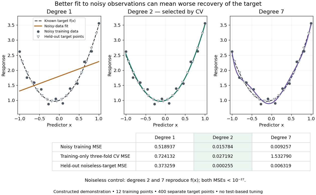
Noisy polynomial fitting, training-only degree selection, and separate noiseless-target evaluation
. Details. 
A neural network composes affine maps with nonlinear activation functions and learns their weights from data.
Cross-validation estimates predictive performance by repeatedly fitting on one part of the data and evaluating on held-out observations. In K-fold cross-validation, divide training data into disjoint folds ; identifies observation 's fold, and is fitted without fold . The displayed average scores each observation using a rule that did not train on it. Weight by observation count when fold sizes differ. Leave-one-out cross-validation uses one observation per fold. [ref]
https://web.stanford.edu/~hastie/ISLR2/Slides/Ch5_Resampling_Methods.pdf. ISLR chapter 5 slides, resampling methods
For the training error example, three folds contain indices with equal remainder modulo 3. Each fit uses eight observations. The squared-error loss averages for degrees 1, 2, and 7 are , , and respectively. Select degree 2 and refit on all twelve training data observations. The folds reuse scarce data while challenging each candidate to predict unseen responses; they do not touch the final test set.
Any learned preprocessing, including variable selection, must also be fitted within each training fold to avoid data leakage. [ref]
https://web.stanford.edu/~hastie/ISLR2/Slides/Ch5_Resampling_Methods.pdf. ISLR chapter 5 slides, the wrong and right way
Repeated tuning can itself overfit the cross-validation score; nested cross-validation uses inner folds for model selection and outer folds for assessment of that entire procedure. [ref]Folds use fewer training observations than the final refit, and their scores are dependent because training observations overlap. [ref]
https://web.stanford.edu/~hastie/ISLR2/Slides/Ch5_Resampling_Methods.pdf. ISLR chapter 5 slides, correlated fold estimates
Splitting must match deployment: for time series forecasting, rolling-origin cross-validation trains on the past and evaluates later observations, preventing future information from entering a forecast. Ordinary random folds need not answer that forecasting question. [ref]For testing one simple hypothesis against another, a test that rejects for sufficiently large likelihood ratio has greatest power among all tests of no greater size.
The score test evaluates the likelihood gradient at the restricted estimator and scales its quadratic form by inverse Fisher information.
A likelihood-ratio test rejects where the alternative likelihood is sufficiently large relative to the null likelihood.
For observed cell counts and null expected counts , the statistic isWith specified null cell probabilities and sufficiently large expected counts, its null limit is .
For a test with rejection region , its power function isIts supremum over the null parameter space is the size of the test.
A joint hypothesis test imposes several parameter restrictions simultaneously and accounts for dependence among their estimators; separate one-parameter confidence intervals do not generally determine its result.
A p-value is the probability, computed under a null hypothesis, of obtaining a test statistic at least as unfavorable to that hypothesis as the observed value.
There are unlisted articles, also show them or only show them.