Error function ($\mathrm{erf}$)

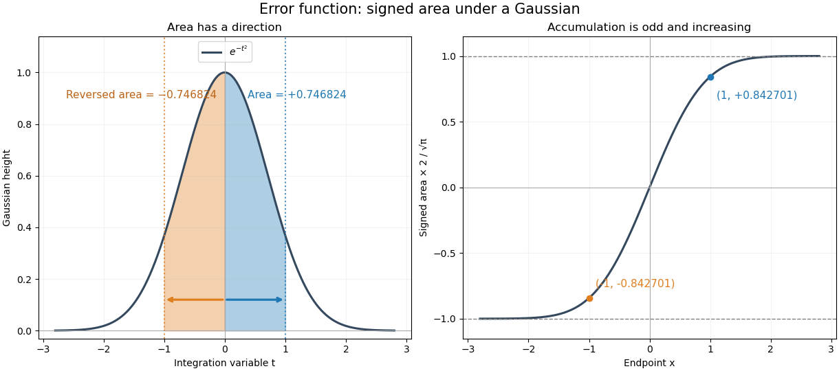
The error function records the signed area under a Gaussian function between zero and a variable endpoint:For a negative real number $x$, reversing the integration limits makes this integral negative. The normalization uses the Gaussian integral: the full area of $e^{-t^2}$ is $\sqrt{\pi }$, so its positive half contributes one after multiplication by $2/\sqrt{\pi }$. The same definition extends to a complex number $z$ along any path from zero to $z$, giving an entire function.^[ref]

For example, $\mathrm{erf}(0)=0$, $\mathrm{erf}(1)\approx 0.842701$, and $\mathrm{erf}(-1)\approx -0.842701$. A finite positive endpoint captures only part of the positive Gaussian integral; $\mathrm{erf}(x)$ approaches one as $x\to +\infty$ but never reaches it at a finite real $x$.

The useful idea is to name a recurring integral once instead of carrying it through every calculation. The error function and the normal distribution express probabilities and quantiles through this area, while an error-function diffusion front describes how diffusion smooths a sharp jump. The complementary error function retains the small area left in the tail.

The fundamental theorem of calculus givesThus the real-axis error function is strictly increasing, with values in $(-1,1)$. Its integrand is an even function, so the error function is an odd function, $\mathrm{erf}(-x)=-\mathrm{erf}(x)$. The derivative also gives ${\mathrm{erf}}^{\prime \prime }(x)=-4x{e}^{-x^2}/\sqrt{\pi }$: the curve is concave for $x>0$ and convex for $x<0$. These real-axis properties do not imply boundedness throughout the complex plane; the existing quadrant asymptotics of the error function describe a different behavior in other directions.

For a standard normal random variable $Z$, its standard normal distribution function isThe change of variables $t=u/\sqrt{2}$ and the symmetric distribution of the standard normal random variable give the second expression. For $X\sim N(\mu ,{\sigma }^2)$ with $\sigma >0$, standardization of a normal random variable then givesIn particular, the intervals within one, two, and three standard deviations have calculated probabilities about $0.682689$, $0.954500$, and $0.997300$. These values depend on a normal distribution; they are not universal coverage guarantees for an arbitrary random variable. This is the direct connection between a Gaussian function area and the familiar central intervals.

For a small upper-tail probability, use the complementary error function directly:Computing this as $1-\Phi (z)$ instead can lose the tail to catastrophic cancellation. The Gaussian tail bound gives another useful estimate without requiring an exact error function value.

Because the real error function is strictly increasing from $-1$ to $1$, its real inverse function maps $(-1,1)$ onto the real line. For $0<q<1$, the standard normal quantile is thereforeMore generally, the $q$-quantile of a normal distribution with expected value $\mu$ and positive standard deviation $\sigma$ is $\mu +\sigma \sqrt{2}{\mathrm{erf}}^{-1}(2q-1)$. This reverses the area calculation: instead of asking how much probability lies below an endpoint, a quantile asks which endpoint encloses a specified probability. The domain restriction matters; $q=0$ and $q=1$ correspond to infinite endpoints, rather than finite real values of the inverse error function.

Consider the one-dimensional diffusion equation on the whole real line,with initial value one for $x<0$ and zero for $x>0$. This is an idealized Heaviside step function profile, not a measured material or an apparatus specification. The heat kernel gives a convolution with the initial profile:The change of variables $s=(x-y)/(2\sqrt{Dt})$ turns the convolution into a Gaussian integral tail. The resulting similarity variable $\eta =x/(2\sqrt{Dt})$ shows that the transition width grows like $\sqrt{Dt}$: multiplying elapsed time by four doubles every fixed-profile distance from the original interface.

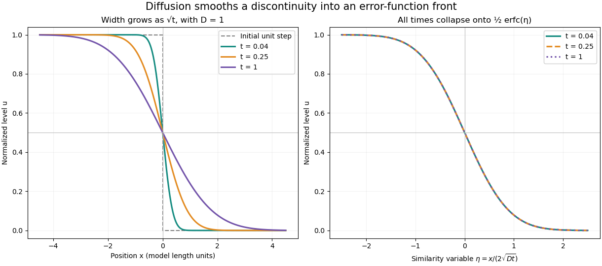
At every positive time, $u(0,t)=1/2$, while $u(x,t)\to 1$ as $x\to -\infty$ and $u(x,t)\to 0$ as $x\to +\infty$. For every fixed $x\ne 0$, the limit as $t\to 0^{+}$ returns the specified initial value. The value assigned at the single initial discontinuity does not change this convolution. The error function therefore explains smoothing without pretending that a discontinuous initial profile remains sharp.

Direct differentiation checks the partial differential equation. Writing $\eta =x/(2\sqrt{Dt})$ givesThe model assumes constant diffusion coefficient, no advection, and no finite-domain boundary effects. For an interpretation as heat conduction, the heat equation applies to a normalized temperature difference under its own material assumptions.

For $z=r{e}^{i\theta }$ with fixed $0\le \theta \le \pi /2$, a horizontal tail gives $f(z)=\sqrt{\pi }/2-e^{-z^2}(2z{)}^{-1}[1+O(z^{-2})]$. The constant dominates through $\theta =\pi /4$; above that angle the exponential endpoint dominates. At the boundary angle its modulus is only $O(r^{-1})$, so the constant remains leading. On the imaginary axis the integral is purely imaginary and grows as $i{e}^{r^2}/(2r)$. The approximation is not a determination of exponentially subdominant constants in that growing sector.

The complementary error function describes the Gaussian integral area remaining beyond the endpoint. For a real $x$,It is an entire function for complex arguments when defined by $1-\mathrm{erf}(z)$. On the real line it decreases from two to zero, with $\mathrm{erfc}(0)=1$ and $\mathrm{erfc}(-x)=2-\mathrm{erfc}(x)$.^[ref]

For example, $\mathrm{erfc}(1)\approx 0.157299$ is a sizeable tail, whereas $\mathrm{erfc}(8)\approx 1.12243\times 10^{-29}$ is extremely small. In the tested floating-point arithmetic, a direct evaluation of $1-\mathrm{erf}(8)$ gives zero because the computed error function has already rounded to one. Evaluating the complementary error function directly preserves this tail. It is the useful quantity in an upper-tail normal distribution probability and in the decaying side of an error-function diffusion front.

For large positive real $x$, the leading asymptotic expansion isThe first corrections are $1-1/(2x^2)+3/(4x^4)-\cdots$ multiplying the leading term. This is an asymptotic expansion, not an assertion that summing arbitrarily many terms converges at a fixed $x$.^[ref] The complementary error function tail bound provides finite-$x$ inequalities instead.

For every real $x>0$,For a short proof, put $I(x)={\int }_x^{\infty }{e}^{-t^2}dt$. Integration by parts givesThe last integral is positive and strictly smaller than $I(x)/x^2$. Using these two inequalities gives the upper and lower bounds after multiplication by $2/\sqrt{\pi }$. Dividing both bounds by $e^{-x^2}/(\sqrt{\pi }x)$ also proves the leading asymptotic equivalence by the squeeze theorem. For small positive $x$, the bounds remain true but can be loose; they are especially useful when the Gaussian integral tail is already small.

The Faddeeva function is an entire function built from the complementary error function. Its integral representation for $\mathrm{Im}z>0$ is $w(z)=(i\pi {)}^{-1}{\int }_{-\infty }^{\infty }{e}^{-t^2}/(t-z)dt$, as normalized in NIST's integral representation. Its reflection identity is $w(-z)=2e^{-z^2}-w(z)$, directly from the odd function property of the error function.

For a pole off the real axis, substitution $s=2t$ into the Faddeeva function integral gives $G(a)=i\pi w(a/2)$ when $\mathrm{Im}a>0$, and $G(a)=-i\pi w(-a/2)$ when $\mathrm{Im}a<0$. The difference of boundary values is the residue theorem jump $2\pi i{e}^{-a^2/4}$. In particular, for a lower-half-plane pole, $G(a)+2\pi i{e}^{-a^2/4}=i\pi w(a/2)$, which packages a crossed residue and a nearby saddle into one smooth expression.