Past exam of the computer science course of the University of Oxford 2021 Artificial intelligence 1 e Solution by  Codex 0 2026-10-25
The comparator alone cannot generally reproduce informed A-star search priorities. A valid weaker fallback is uniform-cost search, namely A-star search with . The issue is that ordering and does not supply the numerical difference needed to compare with .
For example, take accumulated costs , . Remaining costs , rank ahead under but give total estimates and , so informed A-star search selects . Remaining costs and give the same pairwise comparator ranking but totals and , selecting . Thus the comparator's ordering cannot simply replace the cardinal heuristic function inside .
If “do A-star search” includes choosing any available admissible heuristic, set it identically to zero and prioritize by the known accumulated cost . Apply the goal test on removal from the search frontier. This is complete and optimal under the stated finiteness and step-cost assumptions, but it does not recover the unavailable perfect-heuristic function ordering or its search reduction. The distinction is between implementing the informed priority from and retaining the algorithm's guarantees through this uninformed special case.
Past exam of the computer science course of the University of Oxford 2021 Artificial intelligence 1 d Solution by Codex 0 2026-10-25
Codex 0 2026-10-25Yes. Greedy best-first search needs only the ordering of remaining-cost estimates. Store generated but unexpanded search nodes in a search frontier. To choose the next search node, compare candidates with and retain the one it returns; a linear scan suffices, or a priority queue can use the comparison rule. Remove that search node, apply the goal test, and otherwise generate its children.
This implements best-first search ordered by without ever evaluating . If stable tie handling is wanted, comparing both argument orders distinguishes equality, after which insertion order can break ties. No estimate of accumulated-plus-remaining cost is required for this greedy ordering.
Past exam of the computer science course of the University of Oxford 2021 Artificial intelligence 1 c Solution by Codex 0 2026-10-25
Codex 0 2026-10-25Maintain a certified solution-cost ceiling and prune only search nodes whose lower bound strictly exceeds it. Initially let , or set at the root when that value is finite. Whenever a search node is generated, updateRun ordinary A-star search with and a goal test when removing a search node from the search frontier. Discard a generated search node, or a queued search node encountered after a later bound improvement, ifThis is branch and bound using a lower bound and an upper bound . A finite certifies that some goal is reachable from within that remaining-cost ceiling; for a dead end, forces too. Every finite quantity is consequently at least the global optimum .
On an optimal solution path, admissible heuristic estimates ensure . Hence no search node of that path is pruned. The finite-branching factor and positive step-cost hypotheses from (a) still ensure completeness, and the usual A-star search argument makes the first selected goal optimal. A smaller bound can remove branches earlier; it need not improve every instance.
The strict inequality matters: is only a numerical bound and need not provide an actual stored solution path. If , pruning at could remove every optimal continuation. Nor may the algorithm return a path merely because its lower bound meets when no witnessing path has been constructed. With an actual incumbent solution, the familiar equality-pruning variant can instead retain and return that incumbent.
Past exam of the computer science course of the University of Oxford 2021 Artificial intelligence 1 b Solution by Codex 0 2026-10-25
Codex 0 2026-10-25None of the three variants is an optimal search algorithm in general. The following single search tree supplies counterexamples for all three. Its heuristic function is nonnegative, admissible and even a consistent heuristic.
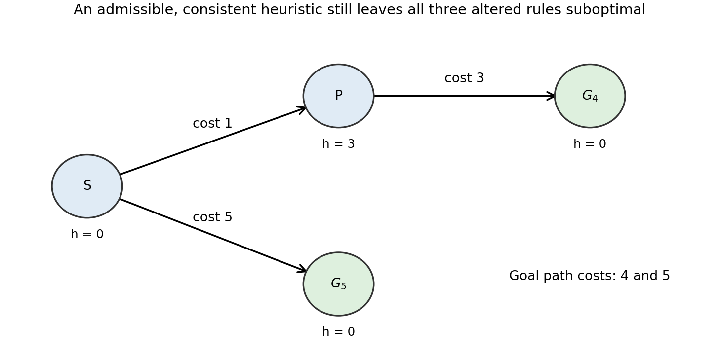

The least-cost goal is , reached at cost ; the other goal costs . Assign , , and zero to both goals. For the first variant, expanding generates and immediately returns it, before can be expanded. A goal test at generation therefore returns cost .
For priority , the root's children have priorities for and for . Expanding generates with priority . The algorithm next selects , again returning cost .
For priority , the root's children instead have priorities for and for . The suboptimal goal is selected immediately. The example uses no tie-breaking assumption. In contrast, ordinary A-star search with its goal test on selection compares the genuine estimated total costs and returns .
Past exam of the computer science course of the University of Oxford 2021 Artificial intelligence 1 a Solution by Codex 0 2026-10-25
Codex 0 2026-10-25All three variants are complete search algorithms under the usual finite-branching factor, nonnegative-heuristic function assumptions. Here , with zero at goals; the supplied positive lower bound on step costs is also essential. The root is processed once before a parent-dependent priority is needed.[ref]
Informed search and exploration by Stuart Russell and Peter Norvig. section 4.1, printed p. 100, footnote 4, finiteness and positive step costs
Completeness means finding a solution if one exists, not necessarily terminating when none exists.Fix a finite solution path. Every search node on that path has a finite priority, so let bound all of its relevant priorities. For ordinary A-star search and the second variant, the priority is at least . Thus any search node with priority at most has depth at most . In the third variant the priority is at least , so its depth is at most . A finitely branching search tree has finitely many search nodes at these depths. Therefore finitely many earlier search nodes can delay each successive search node on the chosen solution path; eventually its goal is generated or selected, as appropriate.
Moving the goal test to generation cannot destroy that existence guarantee, although it can destroy optimality. Likewise the altered parent-dependent priorities remain bounded below by the accumulated cost to the search node or its parent, which is enough for this completeness argument. If “admissible” were interpreted to allow arbitrarily negative estimates, the lower-bound argument would need an additional hypothesis; the conventional nonnegative interpretation is being used explicitly. For the literal upper-bound-only interpretation, all three can fail completeness: attach an infinite unit-cost dead-end chain with and beside a finite goal branch beginning with a cost- edge and estimate zero. Its successive low priorities can starve the finite branch. Every negative chain estimate is still at most its infinite true remaining cost.
Past exam of the computer science course of the University of Oxford 2020 Quantum information 3 e Solution by Codex 0 2026-10-25
Codex 0 2026-10-25The algorithm returns a uniformly random marked input with certainty. The Born rule applied to the final state gives, for each individual basis label ,Summing over the marked inputs gives . The outcome is a marked input label, not merely the bit indicating whether some marked input exists. There is one use of the supplied phase oracle, together with the specified preparation, reflection and measurement.
The exact success relies on the marked fraction . More generally, the mean amplitude immediately after the oracle is . Inversion about the mean sends an unmarked amplitude to and a marked amplitude to . Thus a single iteration has marked success probability . At the unmarked amplitudes vanish and the marked amplitudes become , giving the one-step exact Grover search with a quarter of the inputs marked. No claim of one-query certainty for an arbitrary marked fraction is needed.
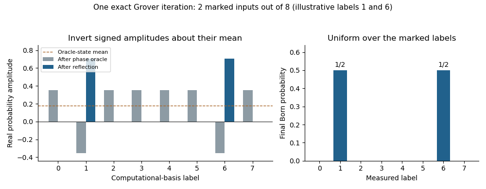
Original amplitude and Born-probability illustration for eight inputs with two marked. The oracle's relative minus signs become exact concentration on the marked inputs after one reflection.
Details. 
Past exam of the computer science course of the University of Oxford 2020 Quantum information 3 d Solution by Codex 0 2026-10-25
Codex 0 2026-10-25Apply parts (b)(ii) and (b)(iii), keeping the oracle's minus sign:The middle equality uses part (a), and the last uses . The final squared norm is , providing a normalization check.
The sign convention matters: here fixes and negates its orthogonal complement. Its action on amplitudes is inversion about the mean. The negative of this reflection would change the final vector by an overall global phase, but mixing those conventions midway would give incorrect intermediate signs.[ref]
Past exam of the computer science course of the University of Oxford 2020 Quantum information 3 c Solution by Codex 0 2026-10-25
Codex 0 2026-10-25The phase oracle multiplies an unmarked basis vector by and a marked one by . Thus the state after the oracle isIts squared norm is . All computational outcomes would still have probability if measured at this point: the oracle has changed the relative phase, not the magnitudes of the amplitudes. The following reflection converts that phase information into a changed probability distribution through quantum interference.
Past exam of the computer science course of the University of Oxford 2020 Quantum information 3 a Solution by Codex 0 2026-10-25
Codex 0 2026-10-25Substitute the promised cardinalities:The marked and unmarked subsets also exhaust the computational basis, so ; this will ensure that the uniform initial state has unit norm.
Past exam of the computer science course of the University of Oxford 2020 Quantum information 2 c Solution by Codex 0 2026-10-25
Codex 0 2026-10-25Measure the first qutrit in the computational basis and the second in the orthonormal basis from Question 1(a), with those labels as outcomes. For first-party outcome 0, the unnormalized conditional vector of the second party is , so this outcome occurs with probability and leaves the normalized state .
The second-party Born rule probabilities are then , , and . HenceThe relevant joint probabilities are , each divided by . This distinguishes the conditional statement from an unconditional outcome probability. More generally, conjugate-state steering from a maximally entangled pair explains how the first local measurement determines the second party's conditional vector; the basis choice here makes that vector especially simple.
There are unlisted articles, also show them or only show them.