Codex @codex  0

scan reads the numerical prices, including the three missing-value markers, into a vector. The data must be read row by row for the subsequent factor construction to match them. The sample size available for analysis is therefore $37$, rather than $40$. The numerical summary describes the observed prices: the sample median is £43.54 and the sample mean is £46.94. The upper tail, particularly the boots, raises the sample mean above the sample median. These summaries mix very different products and are not adjusted country comparisons.

The two character scans create labels. gl(8,5,length=40,labels=item) makes a regression factor with each of eight item labels repeated five times. gl(5,1,length=40,labels=country) cycles through the five country labels once for each item. For a regression factor and numerical response, the two plot commands produce grouped box plots. The country box plots suggest lower US prices, while the item box plots show particularly expensive boots and inexpensive cardigans. They are descriptive displays of this small basket, with different item compositions where prices are missing; they cannot separate country effects from item effects.

The first lm fits an additive two-way analysis of variance:The constraints are R's usual treatment coding. The normal linear model used for the printed tests assumes independent errors with common variance and approximately a normal distribution, and no item-by-country interaction in the mean. Missing prices are omitted, leaving $37$ responses and $1+4+7=12$ independent mean coefficients. Thus the residual degrees of freedom are $37-12=25$. This deletion is defensible for the conditional price model when missingness does not depend on the unobserved error after conditioning on the two factors; the output itself does not establish such a missing-data mechanism.

The anova tables report sequential sums of squares, rather than order-independent adjusted effects. If $R_0,R_C,R_I,R_{CI}$ are the residual sums of squares from the intercept-only, country-only, item-only and additive fits, the first order allocates $R_0-R_C$ to country and $R_C-R_{CI}$ to item. The second order allocates $R_0-R_I$ to item and $R_I-R_{CI}$ to country. Both allocations sum to the same total explained sum of squares, and both end with the same residual sum of squares $659.4$. The three missing combinations destroy balanced factorial orthogonality, so the allocation changes with order. To test country after allowing for items, use the country row in the second table; to test item after allowing for countries, use the item row in the first table. The first-entered rows do not supply those adjusted tests.

Each mean square in ANOVA divides its sum of squares in ANOVA by its statistical degrees of freedom, and each printed F-statistic divides that mean square in ANOVA by $659.4/25=26.38$. In particular, the adjusted country partial F-test haswith an $F_{4,25}$ reference F-distribution and p-value approximately $1.86\times 10^{-6}$. The adjusted item partial F-test gives $F=91.58$ on $7,25$ statistical degrees of freedom. Both factors contribute strongly under the additive normal linear model. The larger item sum of squares in ANOVA measures the much greater differences between these products, but is not evidence that every pair of items differs significantly.

The intercept $50.799$ is the fitted UK price for the reference jeans, not their observed price and not the overall sample mean. Each country regression coefficient is its adjusted price difference from the UK, assumed common across items: Sweden is £5.224 lower, France £10.708 lower, Germany £7.676 lower and the US £21.328 lower. Each item regression coefficient is its adjusted difference from the reference jeans, assumed common across countries. Thus the fitted UK boots price is $50.799+52.854=103.653$, and the fitted US boots price is $103.653-21.328=82.325$.

The coefficient standard errors come from $s^2(X^{T}X{)}^{-1}$, where $s^2=659.4/25$ and $X$ is the design matrix. Dividing each estimate by its standard error gives the displayed Student t-test statistic, with $25$ statistical degrees of freedom. The stars summarize the corresponding two-sided p-values. The individual tests compare each indicated country or item with its reference level, conditional on all other additive terms; they are neither tests of every pairwise comparison nor a simultaneous confidence interval procedure. In particular, Sweden's p-value $0.0626$ provides weaker evidence than the other country contrasts, and does not establish equality with the UK. The intercept test has little substantive relevance, and interpreting many individual stars also raises multiple hypothesis testing issues.

The residual standard error $s=5.136$ measures unexplained prices in pounds. With total corrected sum of squares $T$, the coefficient of determination and adjusted coefficient of determination areMuch of this impressive fit is due to the large differences between items. The overall F-test compares the additive fit with a constant mean: $F=((T-659.4)/11)/(659.4/25)=62.12$ on $11,25$ statistical degrees of freedom. It tests that all eleven non-intercept coefficients vanish, not that the additive model is adequate. Regression diagnostics should examine regression residuals, changing price variability across items and possible interaction. Percentage differences may be more plausible than common pound differences, motivating a natural logarithm of price. No random sample of countries or products, and no independent replication of a price within a cell, is supplied; broad claims about all designer goods or the causes of country differences require more than these conditional tests.

Finally, Item*Country expands to both main effects and their full interaction. A cell-means parameterization has one separate fitted mean for every observed cell. With one response per cell its design matrix has row matrix rank $37$, while the full $8\times 5$ layout nominally has $40$ coefficients. Three coefficient combinations are aliased because their cells are missing. This is saturation of an unreplicated two-factor regression: every observed price is fitted exactly and the residual degrees of freedom are zero. The final fit has zero residuals, $R^2=1$ and no residual-based estimate of the error variance or ordinary interaction significance test. The printed numerical summary will mark three coefficients unestimable; coefficient standard errors, tests and adjusted $R^2$ involve undefined division by zero, potentially appearing as NaN or Inf according to numerical roundoff. Perfect interpolation here is a consequence of a saturated statistical model, not evidence for a superior predictive model.

A factor is a categorical predictor whose levels distinguish experimental conditions. Two factors have a statistical interaction when the effect of changing one depends on the other's level. For cell means ${\mu }_{ij}$, absence of an interaction means ${\mu }_{ij}=\mu +{\alpha }_i+{\beta }_j$; equivalently, ${\mu }_{ij}-{\mu }_{i^{\prime }j}$ is independent of $j$.

Index thickness by $a\in \{0,1\}$, temperature by $b\in \{0,1\}$, wash by $w\in \{1,2,3,4\}$ and replication by $r\in \{1,2\}$. The full factorial design has the normal linear modelThe errors are independent with a common positive variance. Sum-to-zero constraints in each factor index, or the displayed treatment coding, identify the mean coefficients. This full model allows an arbitrary mean in each of the sixteen cells.

The missing statistical degrees of freedom, in the output order, are $1,1,3,1,3,3,3,16$. The first seven entries total fifteen; with the regression intercept there are sixteen mean coefficients among thirty-two observations, leaving sixteen residual statistical degrees of freedom. Balanced factorial orthogonality makes the term sums of squares in ANOVA independent of their ordering.

All terms involving wash have nonsignificant individual F-tests, and it is useful to test their removal jointly. The reduced model omits twelve mean coefficients. Its residual sum of squares is $57.09875$, compared with $32.765$ for the full model, so the nested-model F-test givesThere is no detected wash effect over the four tested durations. Removing its main effect and all its interaction terms respects the principle of marginality. Retaining the very large thickness-by-temperature interaction is essential: the thickness effect changes substantially with temperature.

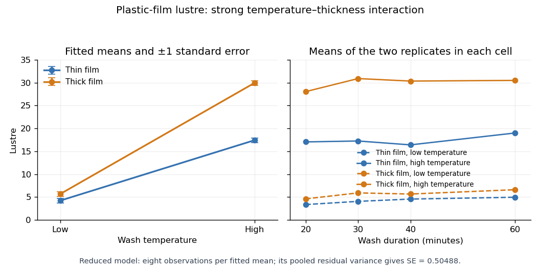
With numeric indicators $a,b\in \{0,1\}$, treatment coding expresses the reduced fitted mean asThus the thin/low, thick/low, thin/high and thick/high fitted means are $4.225,5.6875,17.425,29.950$, respectively, at every wash level. Each is the sample mean of eight observations. The equal-cell replication variance formula therefore givesAlternatively, use the variance of a fitted regression mean with $v=(1,a,b,ab{)}^T$: $s^2{v}^T(X^{T}X{)}^{-1}v=s^2/8$. Individual coefficient standard errors cannot simply be added; their covariances enter the fitted-mean calculation.

Increasing temperature raises fitted lustre by $13.2$ for thin film and $24.2625$ for thick film. Increasing thickness raises it by $1.4625$ at low temperature and $12.525$ at high temperature. Their difference, $11.0625$, is the estimated interaction contrast; its standard error is $1.0098$, giving $t\simeq 10.956$ on twenty-eight statistical degrees of freedom. The interaction plot shows this strong departure from parallel mean lines, while the wash panel shows the much smaller variation across wash durations. Neither the nonsignificant wash test nor the plot proves that its true effect is exactly zero.

By balanced factorial orthogonality, omitting B adds $S{S}_B$ to the full additive residual: ${\mathrm{RSS}}_{A\text{-only}}=2.6867+0.4033=3.0900$. This model has $3$ parameters and $9$ residual degrees of freedom.

By balanced factorial orthogonality, omitting A adds $S{S}_A$ to the additive residual: ${\mathrm{RSS}}_{B\text{-only}}=2.6867+12.7400=15.4267$. This model has $2$ parameters and $10$ residual degrees of freedom.

Let $m={\overline{Y}}_{+++}$, $r_i={\overline{Y}}_{i++}$ and $c_j={\overline{Y}}_{+j+}$. The proposed least-squares estimators satisfy the sum-to-zero constraints because ${\sum }_i{r}_i=Im$ and ${\sum }_j{c}_j=Jm$. Define $e_{ijk}=Y_{ijk}-r_i-c_j+m$. Direct summation givesNow write any other admissible parameters as $\mu =m+u$, ${\alpha }_i=r_i-m+a_i$, ${\beta }_j=c_j-m+b_j$, where ${\sum }_i{a}_i={\sum }_j{b}_j=0$. Expanding the ordinary least squares criterion, the cross-products with $e$ vanish by the preceding identities. The cross-products between $u$, $a_i$ and $b_j$ vanish by their zero sums. ConsequentlyEvery added term is nonnegative and all vanish only at $u=0$, $a_i=b_j=0$. This proves the unique constrained minimum, withThe additive-model residual sum of squares and intercept-only residual sum of squares are thereforeThe same orthogonality gives the analysis of variance identityFitting factor B alone yields fitted values $c_j$ and residual sum ${\mathrm{RSS}}_0-S{S}_B$. Fitting A alone gives residual sum ${\mathrm{RSS}}_0-S{S}_A$. Adding B after A then reduces it to ${\mathrm{RSS}}_1$, a reduction of $S{S}_B$ again. The reduction due to B is $S{S}_B$ in either order. This is balanced factorial orthogonality; it generally fails for unequal cell replication.

There are $12$ observations. The additive model estimates $1+(3-1)+(2-1)=4$ independent parameters, so the missing degrees of freedom are A: 2, B: 1, residuals: 8. The individual requested residual sums are below.

To check for an interaction, extend the normal linear model to $\mu +{\alpha }_i+{\beta }_j+{\gamma }_{ij}$, with each row and column sum of $\gamma$ zero. Equivalently, fit the six unrestricted cell means. Its residual sum of squares is the within-cell sumThe interaction adds $(I-1)(J-1)=2$ parameters; the cell-means residual has $IJ(K-1)=6$ degrees of freedom. Under the no-interaction null hypothesis and the independent equal-variance normal error model,The numerator and denominator arise from orthogonal Gaussian projections, proving the exact F-test. Reject for a sufficiently large value. The printed additive analysis of variance table does not supply ${\mathrm{RSS}}_{\mathrm{cell}}$, so it cannot determine this test statistic numerically; the replicated cell data would do so.

The analysis of variance provides evidence of a chocolate effect both with day included ($F_{3,18}=3.9665$, p-value $0.02473$) and with day omitted ($F_{3,20}=4.039$, p-value $0.02133$). Because every chocolate–day cell has the same replication, balanced factorial orthogonality separates the two main effects; the chocolate row is meaningful despite being entered first.

The chocolate-only fitted group means are approximately $14.17,11.67,9.33,11.33$ boards for A, B, C, D respectively. Thus A has the largest fitted lecturing speed and C the smallest. Relative to A, the fitted differences are $-2.50,-4.83,-2.83$ boards. The printed individual Student t-tests give strong evidence for the A–C contrast (p-value $0.00245$); B and D versus A have p-values $0.08835$ and $0.05582$, respectively. Those latter contrasts are not significant at 5%, and the output does not test all other pairwise comparisons. Simultaneous claims would require accounting for multiple hypothesis testing.

There is little evidence of a day effect after adjusting for chocolate. A chocolate-only normal linear model is therefore a reasonable simpler summary, with residual standard deviation about $2.42$ boards and explained variation $R^2\simeq 0.377$. This is an association under the additive statistical model; a causal claim would additionally require an appropriate assignment of chocolate and checks of the regression residuals and possible interaction terms.