Use for the normal-state single-spin density of states per unit energy and volume at the Fermi surface. Write the attraction as , with , and define .[ref]
Theory of Superconductivity by John Bardeen and others. p.1182, equations (2.34)–(2.40), one-spin density of states; volume normalization stated here
Since has units of energy, has units of energy times volume, making dimensionless. Set , an energy cutoff using the Debye frequency , rather than a frequency itself. These conventions also fix the meaning of the earlier constant-shell BCS gap equation.
Here is the reduction of the BCS gap equation in these conventions. Substituting the zero-temperature BCS anomalous average givesThe sum counts one spin species. For , cancelling and replacing this sum by an integral with constant givesThe factor two from the symmetric integral cancels the in the BCS anomalous average; it is not an extra spin degeneracy. Substituting evaluates the integral as . Solving givesThe first equality is exact within the constant-density of states, sharp-cutoff mean-field approximation; the last is the weak coupling asymptote. Extending the first equality to large does not make this simplified model an accurate description of a strongly coupled material.
For an original numerical example, choose and . The exact constant-shell BCS gap equation gives ; the weak coupling formula gives . Its fractional underestimate, measured against the exact result, is exactly . At that error is , so the two formulas are no longer interchangeable. No material parameters have been fitted here.
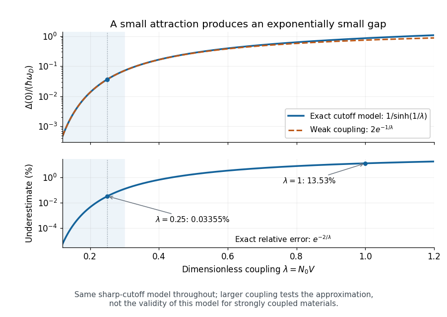
The exact cutoff gap and the range of the weak-coupling approximation
. Original zero-temperature constant-shell BCS gap equation calculation. The upper panel compares with ; the lower panel gives the exact fractional underestimate . The shaded interval is a chosen small-coupling illustration, not an experimental boundary. The large-coupling part tests the asymptote within the same model. Details.
At nonzero temperature, substitute the finite-temperature BCS anomalous average instead. The same cancellation yieldsAt the superconducting transition temperature take the continuous limit. The integrand at then has the finite limiting value , so no divergent endpoint needs to be inserted into a numerical quadrature. For , the resulting integral gives and . These ratios concern the isotropic weak coupling model.[ref]
Microscopic Quantum Interference Effects in the Theory of Superconductivity by Leon Neil Cooper. 1972 lecture, thermodynamic properties of the ideal superconductor, pp.80–82
Articles by others on the same topic
There are currently no matching articles.