Bernoulli corrections for polynomial sums (${\sum }_{k=1}^N{k}^4=\frac{N^5}{5}+\frac{N^4}{2}+\frac{N^3}{3}-\frac{N}{30}$)

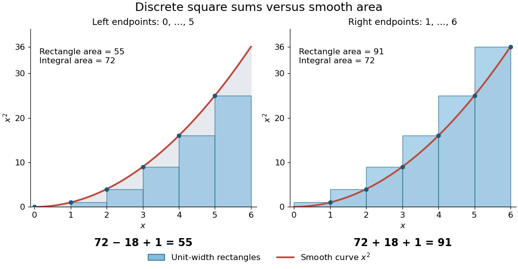
For a concrete comparison, take $f(x)=x^2$ on $[0,6]$. The integral is $I={\int }_0^6{x}^{2}dx=72$, whereas the unit-width left and right Riemann sums are $L=55$ and $R=91$. The exact integer power sum formula givesThe endpoint choice explains the opposite signs of the $18$ correction. The remaining correction is one in both cases.

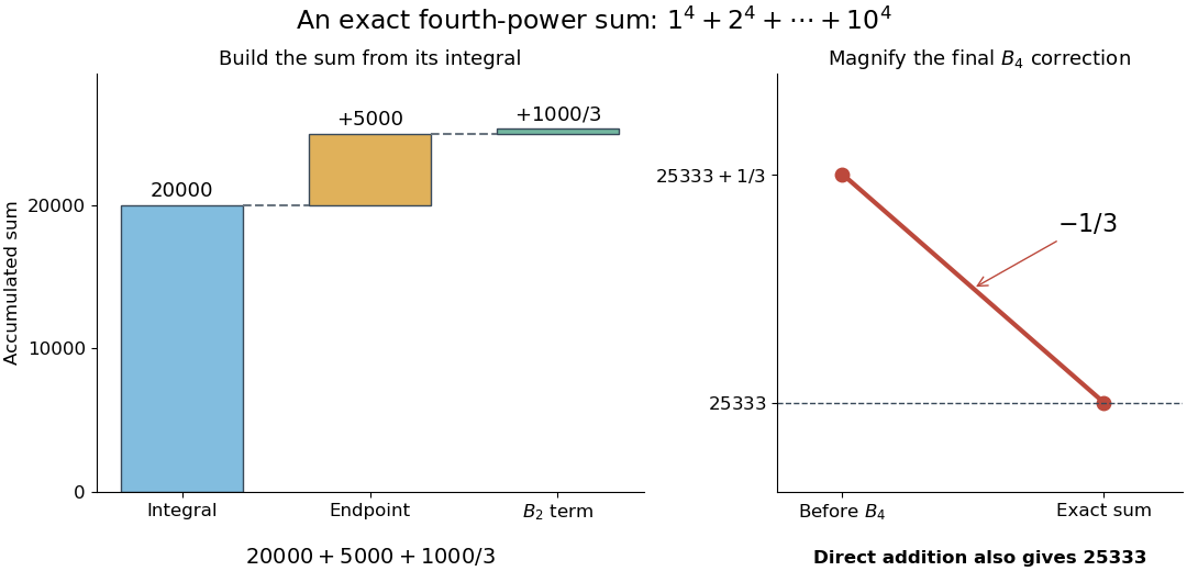
The same method is useful far beyond squares of numbers. Substituting $B_0$, $B_1$, $B_2$ and $B_4$ into the integer power sum formula gives the exact fourth-power resultAt $N=10$, this isThus a finite polynomial calculation replaces ten additions, or a million additions if $N$ is a million. Although the individual corrections can be rational numbers, the result is the exact integer sum.

There is also a useful numerical integration interpretation. The average of the left and right Riemann sums is the composite trapezoidal rule. For $x^2$, the endpoint corrections cancel but its value is $73$, one above the true integral. Subtracting the $B_2$ correction makes this particular polynomial example exact. For $f(x)=x^4$, the two interior corrections above can be written $B_2(f^{\prime }(N)-f^{\prime }(0))/2!$ and $B_4(f^{\prime \prime \prime }(N)-f^{\prime \prime \prime }(0))/4!$. These are exact identities for these polynomials; extending such corrections to general functions requires a separate error analysis.