As a quadrature rule, the trapezoidal rule replaces an integrand by the linear interpolation joining its two endpoint values:For nonnegative endpoint values, this is the area of a trapezoid; in general it is a signed area. The quadrature nodes are , each with quadrature weight . Unlike the midpoint quadrature rule, it uses endpoint samples, which can be reused between adjacent panels.
Every affine function agrees with its linear interpolation, so the trapezoidal rule integrates it exactly. On , gives . On , the polynomial instead gives , exceeding by . Its degree of precision of a quadrature rule is exactly one.
If , its signed approximation error satisfiesA convex function lies below its endpoint chord, so the trapezoidal rule overestimates its integral; a concave function gives the reverse inequality. The error formula assumes that the second derivative exists and is a continuous function throughout the closed interval.[ref]
3.5 Quadrature, subsection (i) Trapezoidal Rules. §3.5(i), equation 3.5.1 and its C² hypothesis; the source writes integral minus rule
A short derivation is the identityobtained by two integrations by parts. The nonnegative Peano kernel has integral , and the weighted mean value theorem for integrals gives the formula.The trapezoidal rule for an ordinary differential equation averages vector fields at the old and new states and is A-stable.
This time-stepping use applies the same trapezoidal rule to the integral of the derivative in an ordinary differential equation. That connection explains its place under implicit Runge-Kutta methods; its quadrature behavior and the nonlinear issue in trapezoidal rule fails B-stability concern different uses of the same endpoint averaging.
For with , the trapezoidal rule satisfies the displayed bound, and the constant is best possible. The polynomial interpolation error for the endpoint linear interpolant satisfies , where . Integrating this inequality and using the triangle inequality for an integral proves the bound because . Equality holds for : the exact integral is , its trapezoidal rule estimate is , and .
On an equal-panel partition of an interval, with , sum the trapezoidal rule over adjacent panels:There are distinct quadrature nodes. Each interior sample belongs to two panels and therefore has quadrature weight , while each endpoint has quadrature weight . Equivalently, the composite trapezoidal rule integrates the piecewise linear function obtained by linear interpolation exactly.[ref]
For and , summing panel quadrature errors givesfor some . Thus panel quadrature errors of order accumulate to order , using big O notation.[ref]
3.5 Quadrature, subsection (i) Trapezoidal Rules. §3.5(i), equations 3.5.2–3.5.3: composite formula and signed error
On a nonuniform partition of an interval with widths and largest width , the bound is .For the polynomial on , direct summation yieldsBoth quadrature errors shrink by exactly four when doubles, with opposite signs. This exact relation belongs to this polynomial example; the trapezoidal rule is not always twice as inaccurate as the midpoint quadrature rule.
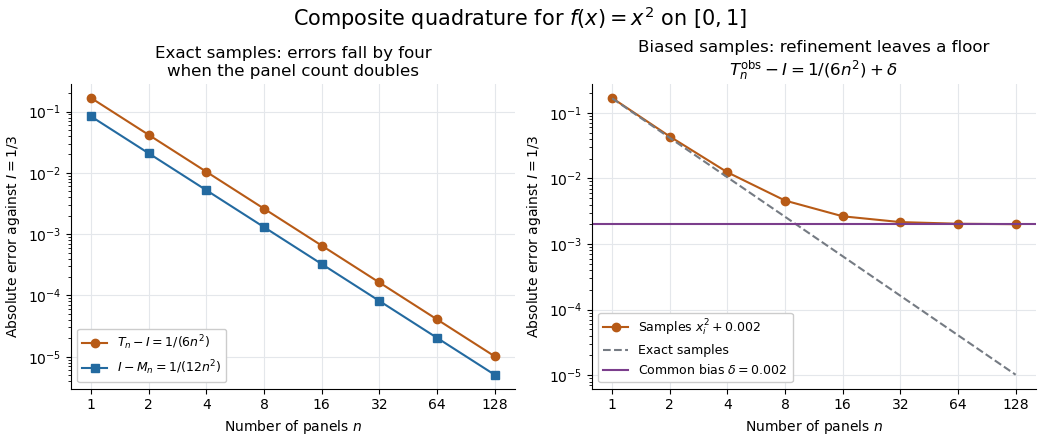
Quadratic quadrature errors fall by four on refinement while a common sample bias persists
. Details. 
The left plot uses exact polynomial sums; the right adds a common sample bias to the composite trapezoidal rule. That mathematical model converges to , showing why smaller panels alone do not ensure accuracy for noisy samples. It illustrates noise sensitivity of a quadrature rule, rather than measured data.
On a partition of an interval symmetric about zero, the composite trapezoidal rule gives opposite quadrature nodes equal quadrature weights. Samples of an odd function cancel pairwise, and a zero quadrature node contributes zero. For a continuous odd function, its exact integral over is also zero. Adding any affine function preserves exactness by linearity of the integral and of the quadrature rule. For example, is nonpolynomial but both the exact integral and every uniform-grid composite trapezoidal rule value on are two.
On a uniform partition of with width , the right Riemann sum and the composite trapezoidal rule have equal weights at every interior mesh point. They differ only by adding half a final-endpoint weight and removing half an initial-endpoint weight. This proves the displayed identity. For continuous , both converge to its definite integral; their finite endpoint correction need not be confused with the smaller trapezoidal discretization error for a smooth integrand.
If is twice continuously differentiable on , take a uniform bound . On one panel , two integrations by parts give the signed quadrature errorThe nonnegative kernel has integral , so the absolute error is at most . Summing equal panels proves the displayed bound. The maximum exists on the closed interval; a supremum or any known uniform bound also suffices. The estimate certifies a sufficient panel count, which need not be the least count achieving a particular actual error.
The trapezoidal rule is A-stable but is not B-stable. For the dissipative vector field at step size one, its uniquely defined step map obeys . At , and implicit differentiation gives , so nearby states expand rather than contract. This is a concrete nonlinear obstruction, rather than merely failure of the sufficient algebraic stability criterion.
Articles by others on the same topic
There are currently no matching articles.