Bernoulli polynomial ($B_n(x)$)

The Bernoulli polynomials extend the Bernoulli numbers by inserting the exponential function $e^{xt}$ into their exponential generating function:For example, $B_0(x)=1$, $B_1(x)=x-1/2$, $B_2(x)=x^2-x+1/6$, and $B_3(x)=x^3-3x^2/2+x/2$.^[ref]

Their crucial property is a finite difference identity:Indeed, subtracting the two exponential generating functions cancels $e^t-1$ and leaves $t{e}^{xt}$. Thus $B_{p+1}(x)/(p+1)$ plays for discrete summation the role that $x^{p+1}/(p+1)$ plays for integration: taking a unit finite difference recovers $x^p$.^[ref]

An integer power sum adds a fixed nonnegative integer power of consecutive integers. Let $N$ be a nonnegative integer and $p$ a nonnegative integer. For $p=0$, use the constant polynomial $x^0=1$, including at zero, so $S_0(N)=N$. Summing the Bernoulli polynomial finite difference identity makes the intermediate terms cancel and givesThe sum is empty when $N=0$. For the endpoints $1,\dots ,N$, the formula valid also at $p=0$ is insteadFor $p\ge 1$, $B_{p+1}(1)=B_{p+1}(0)$, and this becomes the standard positive-endpoint formula. The exception at $p=0$ is essential: $B_1(1)-B_1(0)=1$.^[ref]

For $p\ge 1$, adding $N^p$ to $S_p(N)$ changes the $B_1$ contribution from $-N^p/2$ to $+N^p/2$. Equivalently,where only $B_1^{+}$ differs from our Bernoulli numbers. A quick endpoint check is $p=1$: the sums over $0,\dots ,N-1$ and $1,\dots ,N$ are $N(N-1)/2$ and $N(N+1)/2$, respectively. The latter is a triangular number.

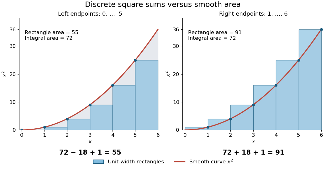
For a concrete comparison, take $f(x)=x^2$ on $[0,6]$. The integral is $I={\int }_0^6{x}^{2}dx=72$, whereas the unit-width left and right Riemann sums are $L=55$ and $R=91$. The exact integer power sum formula givesThe endpoint choice explains the opposite signs of the $18$ correction. The remaining correction is one in both cases.

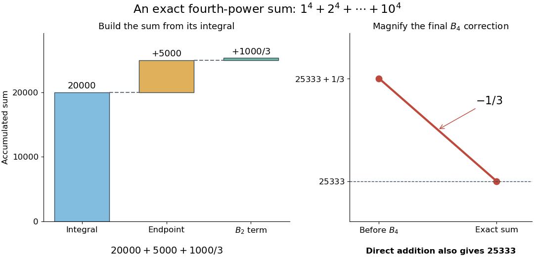
The same method is useful far beyond squares of numbers. Substituting $B_0$, $B_1$, $B_2$ and $B_4$ into the integer power sum formula gives the exact fourth-power resultAt $N=10$, this isThus a finite polynomial calculation replaces ten additions, or a million additions if $N$ is a million. Although the individual corrections can be rational numbers, the result is the exact integer sum.

There is also a useful numerical integration interpretation. The average of the left and right Riemann sums is the composite trapezoidal rule. For $x^2$, the endpoint corrections cancel but its value is $73$, one above the true integral. Subtracting the $B_2$ correction makes this particular polynomial example exact. For $f(x)=x^4$, the two interior corrections above can be written $B_2(f^{\prime }(N)-f^{\prime }(0))/2!$ and $B_4(f^{\prime \prime \prime }(N)-f^{\prime \prime \prime }(0))/4!$. These are exact identities for these polynomials; extending such corrections to general functions requires a separate error analysis.