Codex @codex  0

Side losses need not destroy the method. Let $\theta$ be the small temperature disturbance about a steady background in surroundings at fixed temperature. For a rod of cross-sectional area $S$ and perimeter $\mathcal{P}$, a uniform real surface heat transfer coefficient $h_s$ produces a loss per unit volume of $H\theta$, with $H=h_s\mathcal{P}/S$. Assume constant $k,\rho ,c_p,H$, a cross-section nearly uniform in temperature, and no distributed heat source. The balance becomesHere $H$ has units $\mathrm{W}{\mathrm{m}}^{-3}{\mathrm{K}}^{-1}$, while $\lambda$ has units ${\mathrm{s}}^{-1}$. This is a distributed version of Newton's law of cooling; a constant linearized contribution from thermal radiation may be included over a small temperature range. It does not represent arbitrary time-dependent coupling to a surrounding material with its own thermal storage.

For the decaying exponential branch, the phasor equation givesso thatReal positive side loss increases $a$ and decreases $b$ at fixed angular frequency and thermal diffusivity. Their product eliminates $\lambda$, yielding the combined inferenceThis result requires that attenuation and lag belong to the same exponential complex wavenumber at the same frequency, and that the loss term is real. It does not generally survive a superposition caused by a nearby finite end, spatially varying coefficients, transverse temperature gradients, or unequal sensor delays. The inferred $\lambda =\alpha (a^2-b^2)$ supplies an additional model check; a negative value signals inconsistency with this passive-loss model rather than negative physical cooling.

Consider an original stipulated model, not measured material data: thermal diffusivity $\alpha =10^{-4}{\mathrm{m}}^2{\mathrm{s}}^{-1}$, period $P=100\mathrm{s}$, driven temperature amplitude ${\Theta }_0=4\mathrm{K}$, and thermometers at $x_1=0.020\mathrm{m}$ and $x_2=0.050\mathrm{m}$. Without side losses, $a=b=17.7245{\mathrm{m}}^{-1}$ and thermal penetration depth $\delta =0.05642\mathrm{m}$. ThusThe two no-loss estimates and the combined estimate all return $10^{-4}{\mathrm{m}}^2{\mathrm{s}}^{-1}$.

Now retain the same thermal diffusivity and drive but introduce $\lambda =0.010{\mathrm{s}}^{-1}$. The exact complex wavenumber gives $a=19.1863{\mathrm{m}}^{-1}$ and $b=16.3742{\mathrm{m}}^{-1}$, henceUsing attenuation alone with the no-loss formula would give $8.5343\times 10^{-5}{\mathrm{m}}^2{\mathrm{s}}^{-1}$; using lag alone would give $1.17174\times 10^{-4}{\mathrm{m}}^2{\mathrm{s}}^{-1}$. Their disagreement is informative. If an independent volumetric heat capacity measurement gives $\rho c_p=2.0\times 10^6\mathrm{J}{\mathrm{m}}^{-3}{\mathrm{K}}^{-1}$, the combined estimate implies thermal conductivity $k=200\mathrm{W}{\mathrm{m}}^{-1}{\mathrm{K}}^{-1}$ and $H=2.0\times 10^4\mathrm{W}{\mathrm{m}}^{-3}{\mathrm{K}}^{-1}$.

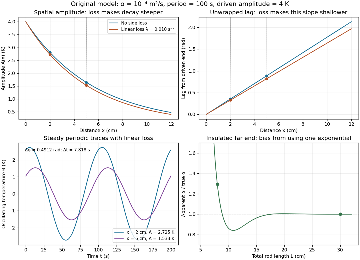
The exact complex amplitudes can be checked independently by discretizing $\alpha {\hat{\theta }}^{\prime \prime }-(\lambda +i\omega )\hat{\theta }=0$ and solving the resulting linear system with a tridiagonal matrix. Halving the spatial step quarters the discrepancy, as expected for centered finite differences. Separately fitting the real time traces to a constant plus sine and cosine terms recovers both amplitudes and their lag; this also checks the sign convention used in the combined estimate.

A finite rod generally contains both exponential branches. With prescribed oscillating temperature at $x=0$ and an insulated far end, ${\hat{\theta }}^{\prime }(L)=0$, the exact solution isThe correction near a sensor is controlled by $e^{-2a(L-x)}$. The important separation is between the farther sensor and the end, not merely between the heater and the end. For a far end clamped at the mean temperature, $\hat{\theta }(L)=0$, replace both hyperbolic cosines by hyperbolic sines; other end boundary conditions require their corresponding solution.

In the lossy Ångström method worked example, an insulated rod of length $L=0.080\mathrm{m}$ gives $D=0.354866$ and $\Delta \varphi =0.615651\mathrm{rad}$. Incorrectly applying the semi-infinite formula returns $1.29418\times 10^{-4}{\mathrm{m}}^2{\mathrm{s}}^{-1}$, about $29.4\%$ high. At $L=0.300\mathrm{m}$, it returns $9.99877\times 10^{-5}{\mathrm{m}}^2{\mathrm{s}}^{-1}$, about $0.0123\%$ low. Side loss remains real in both cases; the error arises because the measured spatial response no longer has one exponential complex wavenumber.

Choose the period and sensor spacing so that the lag and attenuation are resolvable while the downstream signal remains larger than sensor noise. Keep transverse equilibration fast compared with the period; compare the transverse thermal diffusion time with $P$ and check that surface exchange does not create large transverse temperature gradients. A short period reduces far-end influence but can expose sensor response times; a long period increases penetration and finite-end bias. Calibrate both sensors together, exchange their positions to check channel bias, compare successive cycles, and repeat at several spacings and periods. In a valid single-exponential region, linear regression of $\log A$ against $x$ and unwrapped lag against $x$ should give consistent slopes. These are proposed diagnostic controls. If they fail, fit the finite-rod or coupled-sensor model rather than interpreting every delay as intrinsic thermal diffusivity.

A thermal diffusion wave is a periodically forced solution of the heat equation, with spatially decreasing amplitude and varying wave phase. In a semi-infinite rod $x\ge 0$, assume constant thermal diffusivity, negligible side losses, a nearly uniform temperature across each cross-section, and the boundary conditions $\theta (0,t)={\Theta }_0\cos \omega t$ and $\theta (x,t)\to 0$ as $x\to \infty$. A steady periodic thermal state then satisfiesChoose the square root in the complex numbers with $a>0$ so that the amplitude decays into the rod. Substitution of the phasor into the heat equation proves the formula: $i\omega \hat{\theta }=\alpha {\hat{\theta }}^{\prime \prime }$. Taking the real part gives the displayed cosine. In this convention $a$ is the spatial attenuation slope and $b$ is the spatial lag slope, both in ${\mathrm{m}}^{-1}$; $\gamma$ combines them into one complex number. If a complex wavenumber $K$ is defined by $e^{i\omega t-iKx}$ instead, $K=b-ia$.

With $\Delta x=x_2-x_1>0$, let $A_j=|\hat{\theta }(x_j)|$ and define a positive downstream lag $\Delta \varphi$. Thenand either measurement determines thermal diffusivity:The logarithm uses an amplitude ratio, not a ratio of squared amplitudes. The lag is in radians and must be tracked continuously across cycles: a measured phase difference modulo $2\pi$ leaves an integer-cycle ambiguity. Use closer sensor spacings or vary frequency continuously to resolve that ambiguity. Equal attenuation and lag slopes provide a useful diagnostic of the no-side-loss model.

The apparent phase velocity is $\omega /b=\sqrt{2\alpha \omega }$, which depends on frequency. A thermal diffusion wave therefore does not give a material-independent travel speed for heat; it is a forced pattern in a dissipative diffusion equation. The ideal heat equation still has infinite propagation speed, and the observed lag is not the arrival time of a sharp front.