A thermometer measures temperature through a physical response whose relation to temperature is known. Examples include the length change from thermal expansion, a change in electrical resistance, and the pressure of a gas thermometer. If the response function is an injective function over the working range, its measured value determines through the inverse function. Thermometer calibration establishes that relation for the particular instrument and measurement conditions. Two matching readings are meaningful only after calibration to a common scale and with the probes sampling comparable equilibrium states. [ref]
https://openstax.org/books/university-physics-volume-2/pages/1-2-thermometers-and-temperature-scales. Ling, Moebs and Sanny, University Physics Volume 2, section 1.2: physical responses used in thermometers
For a contact thermometer, the sensing part must reach thermal equilibrium with the region being measured. That region may differ from the rest of the object: an immersed probe near a heater can read a local temperature while the surrounding water remains cooler. A stable reading can also be a steady state set by competing heat transfer paths to the sample and the room. Good contact, adequate immersion, mixing where appropriate, and checks for spatial differences help establish which temperature the reading represents. These are measurement controls inferred from the thermal equilibrium requirement, not a guarantee that every flat trace is equilibrium.
A thermometer also changes the sample it touches. Consider an original toy calculation with an initially uniform sample at , a probe at , and constant whole-body heat capacities and . Suppose together they form an isolated system, with no work or phase transition and negligible contact energy. The first law of thermodynamics and thermal equilibrium giveThe final thermometer reading underestimates the sample's original temperature by about , although it correctly measures their new common temperature. The disturbance becomes small when the participating probe heat capacity is small compared with the sample's. A large controlled heat bath is a different limit: it supplies or removes heat while approximately maintaining its own temperature.
Waiting time is a separate issue from disturbance. Under a toy Newton's law of cooling model for a uniform probe in a maintained heat bath, a constant contact conductance givesThe time constant controls this exponential decay. For stipulated values , and , the probe reads about after one time constant and after three. These are calculated values, not an instrument specification or measured data. Real probes may have multiple relaxation times and additional heat transfer paths; choose an equilibration criterion from the required accuracy, rather than assuming that a fixed waiting time works universally.
A thermometer using differential thermal expansion of a liquid and its glass container to move a column through a calibrated capillary.
A bulb-volume change shifts the indicated temperature. Contraction raises the liquid column at a fixed temperature; expansion lowers it. Permanent and temporary changes require distinction when interpreting an ice-point check.[ref]
A thermometer that infers temperature from a calibrated electrical resistance. Measuring current can heat its sensing element; extrapolation toward zero current controls that bias in the saturation-pressure equilibrium measurement.
A resistance thermometer using platinum as its sensing material. It provides the temperature readout in the saturation-pressure equilibrium measurement.
Transduction turns electrical resistance into a temperature indication. A uniform wire has , with electrical resistivity , length , and cross-sectional area . Stronger atomic vibrations at higher temperature scatter electrons more, increasing platinum's electrical resistivity; impurities and crystallographic defects also contribute.[ref]
Guide on Secondary Thermometry: Industrial Platinum Resistance Thermometers by Jonathan Pearce and others. Guide on Secondary Thermometry: Industrial Platinum Resistance Thermometers, §2.1, printed pp. 6–7: resistivity, electron scattering, and impurities
A small known electric current and measured electric potential difference give through Ohm's law; a resistance bridge can instead compare the element with a reference resistor. Inverting the calibrated response then gives the sensing element's temperature. This makes electrical readout convenient, but the platinum resistance thermometer lead resistance error, resistance thermometer self-heating, and resistance thermometer immersion test explain why a stable display alone is insufficient. The gas thermometer supplies a contrasting route through an equation of state; the saturation-pressure equilibrium measurement shows why a trustworthy independent temperature readout matters.
A standard platinum resistance thermometer uses very pure, annealed platinum with strain-limiting construction. An industrial platinum resistance thermometer commonly uses supported wire or a film. Their response curves differ.[ref]
The word standard describes the instrument's metrological role. Calibrated SPRTs realize specified interpolation intervals of the International Temperature Scale of 1990 and transfer reference temperatures to other thermometers.[ref]
Mercury Thermometer Alternatives: Platinum Resistance Thermometers (PRTs) by National Institute of Standards and Technology. Platinum Resistance Thermometers, opening explanation: SPRTs as ITS-90 interpolation tools
They are primary standards for realizing that practical scale, but their electrical resistance alone does not determine absolute thermodynamic temperature without calibration. Primary thermometry such as the corrected gas thermometer obtains thermodynamic temperature from a physical law. A reference in a comparison bath may be an SPRT; an individually calibrated industrial platinum resistance thermometer can also serve as a working reference with an appropriate uncertainty.An industrial platinum resistance thermometer is a platinum resistance thermometer built for practical measurement conditions. The label Pt100 specifies a nominal reference electrical resistance, not an SPRT, a calibration certificate, or a universal accuracy. Calibrate the probe together with its readout when the desired result is the performance of the complete indicating system.
A Pt100 has nominal electrical resistance at .[ref]
Mercury Thermometer Alternatives: Platinum Resistance Thermometers (PRTs) by National Institute of Standards and Technology. Platinum Resistance Thermometers, opening explanation: conventional 100-ohm element at 0 °C
Here is the reference for the nominal element designation; it is distinct from the water triple point used in SPRT calibration. The following Pt100 local linear model deliberately stipulates one approximate response for calculations.Choose the illustrative local modelHere is the Celsius temperature, measured relative to , so is dimensionless. For this chosen affine function, the derivative and inverse relation areCalculated values are , , , and . These are model outputs, not measurements or an assertion that any real Pt100 follows this line exactly. The number here is the chosen slope parameter; it is not a universal local derivative for all platinum resistance thermometers. Curvature, manufacturing differences, and the fitted calibration interval matter. A wider-range calibration uses a validated response curve rather than extrapolating this line indefinitely.
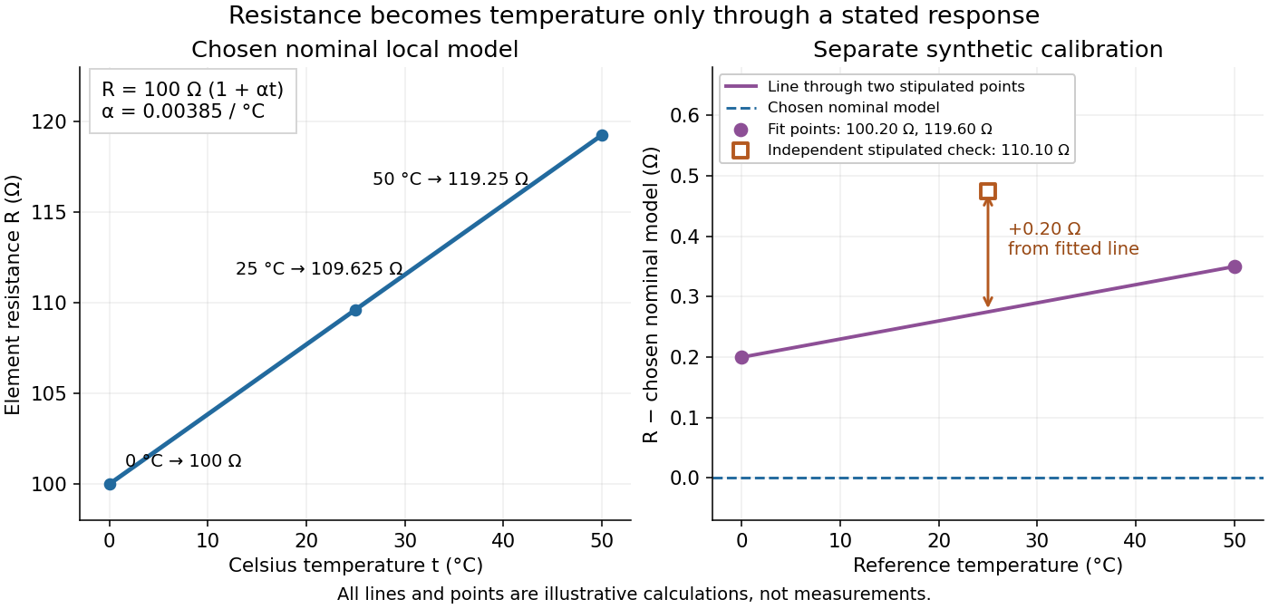
Chosen Pt100 line and an illustrative calibration with an independent check
. The left panel plots the Pt100 local linear model. The right panel uses stipulated values for a different illustrative element: two points set a line, while a third point tests it. Every point is synthetic; none is measured calibration data or a tolerance band. Source. Details.For a separate synthetic thermometer calibration, stipulate at and at . A two-point affine function has slope and givesThus would indicate . If an additional synthetic check at reference instead supplied , the line would indicate . The residual exposes disagreement that two fitted points cannot reveal. This separate example changes both offset and slope; it is not a replacement specification for the nominal Pt100 local linear model.
A 1998 NIST account describes stirred comparison baths, a reference SPRT with a 30 Hz resistance bridge, and a temperature-controlled reference resistor. The test IPRTs used a current source, a scanner, and an 8½-digit voltmeter. Separate current and voltage leads made each test probe a four-terminal device; readings in both current directions supplied voltage ratios to the reference resistor.[ref]
A New NIST Automated Calibration System for Industrial-Grade Platinum Resistance Thermometers by Gregory F. Strouse and others. A New NIST Automated Calibration System for Industrial-Grade Platinum Resistance Thermometers, §§3.1, 3.3 and 4.2, printed pp. 2–6: baths, readout, four-terminal devices and reversed current
Its program bracketed test readings with reference SPRT readings and repeated a block if bath drift was excessive. A check SPRT monitored the system; reference water-triple point measurements checked stability. Sensor depths were matched, and unfamiliar probes underwent immersion tests. Ice and water-triple point readings before and after calibration checked changes. Additional points could test the fitted curve. Reported calibration uncertainties excluded transport, subsequent drift, hysteresis, and the user's measurement system. These are controls and limits of that documented apparatus, not an accuracy promise for all platinum resistance thermometers.[ref]
The inference is a pair: reference temperature from the SPRT, test electrical resistance from the electrical readout. Record measuring electric current, wiring, immersion, and the stated reference scale with each pair. A bath controller's setpoint is not itself the calibrated reference temperature. Returning to a reference and checking intermediate points distinguishes a fitted relation from a reproducible calibration over the intended interval.
With two shared leads of electrical resistances , Ohm's law givesUsing the Pt100 local linear model, positive lead electrical resistance appears as a warmer temperature. At true , stipulated leads of each change into , producing : a calculated bias of about . Subtracting a measured loop correction works only while that loop electrical resistance remains appropriate; cable temperature changes can invalidate it.
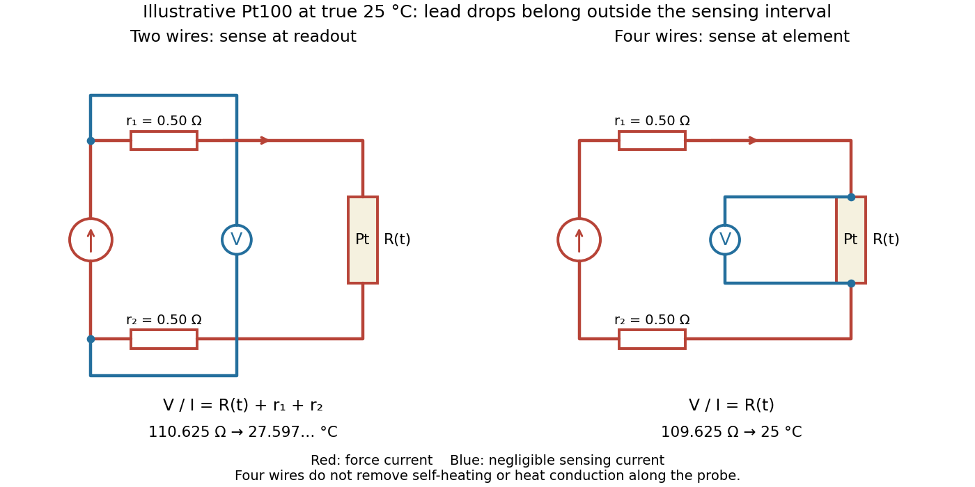
Four-terminal sensing separates the electric current and electric potential difference leads. Negligible sensing electric current suppresses sensing-lead drops; force-lead drops lie outside the interval. Real voltmeter loading, connections, and leakage still need checking.[ref]
For a stable offset from the thermoelectric effect, two signed electric potential differences obey and . The current-reversal calculation in four-terminal sensing yieldsAt stipulated , and , and recover exactly in this model. If the offset or sample temperature changes between readings, cancellation is incomplete. Reversal also leaves Joule heating unchanged because it depends on .
Measuring electric current creates Joule heating, raising the sensing temperature. At fixed bath temperature, compare settled readings at and and extrapolate the approximately linear dependence toward zero current.[ref]
Guide on Secondary Thermometry: Industrial Platinum Resistance Thermometers by Jonathan Pearce and others. §4.1, printed pp. 24–26, equation (4.1.1): self-heating, two-current extrapolation, and medium dependence
Under the local model ,For synthetic readings at and at , the extrapolated value is . The lower-current excess corresponds to in the Pt100 local linear model. At , dissipates ; power alone does not specify a temperature rise without a thermal coupling model. These stipulated values are not measurements.
Repeat the comparison after settling and test the approximation if necessary. Changing from liquid to air changes heat transfer; a self-heating correction need not transfer unchanged. The saturation-pressure equilibrium measurement provides an existing example of controlling this disturbance in resistance thermometry.
A probe's sheath and leads carry heat between the sensing region and the surroundings through thermal conduction. In a stable, sufficiently uniform heat bath, compare the indicated temperature as insertion depth increases, allowing settling each time. A plateau supports adequate immersion for that apparatus and required uncertainty; it does not prove that every depth or medium works. Keep the sensing element and reference thermometer at comparable depths, and check bath gradients independently, so moving the probe does not merely sample a different temperature. The documented platinum resistance thermometer comparison calibration includes these controls.
A thermistor is a temperature-sensitive resistor used as a resistance thermometer. Its calibrated electrical resistance supplies a temperature indication; probe heat capacity and unwanted thermal conduction can affect its response and immersion error.
A gas thermometer infers temperature from the equation of state of a confined gas. The constant-volume version measures pressure; the constant-pressure version measures volume. For an ideal gas,Here is particle number, is amount of substance, is the Boltzmann constant, and is the molar gas constant. The reference and test states must be internally equilibrated, and must be known on the absolute thermodynamic temperature scale. A pressure ratio cancels the unknown gas inventory and bulb size in the ideal constant-volume limit. This cancellation is the method's appeal: a mechanical measurement transfers an absolute temperature scale between different materials. The Maxwell speed distribution and ideal gas pressure from wall collisions explain the microscopic origin of the response. [ref]
2.1 Molecular Model of an Ideal Gas. OpenStax, University Physics Volume 2, section 2.1: the ideal gas law
For an original ideal-model calculation, choose , and . Then . These are stipulated values, not observations. Both pressures must be absolute, referred to vacuum. If the surrounding atmospheric pressure were , the corresponding gauge pressures would be and ; their ratio is three, which would incorrectly predict . A pressure difference from the atmosphere cannot be substituted into the ideal gas law.
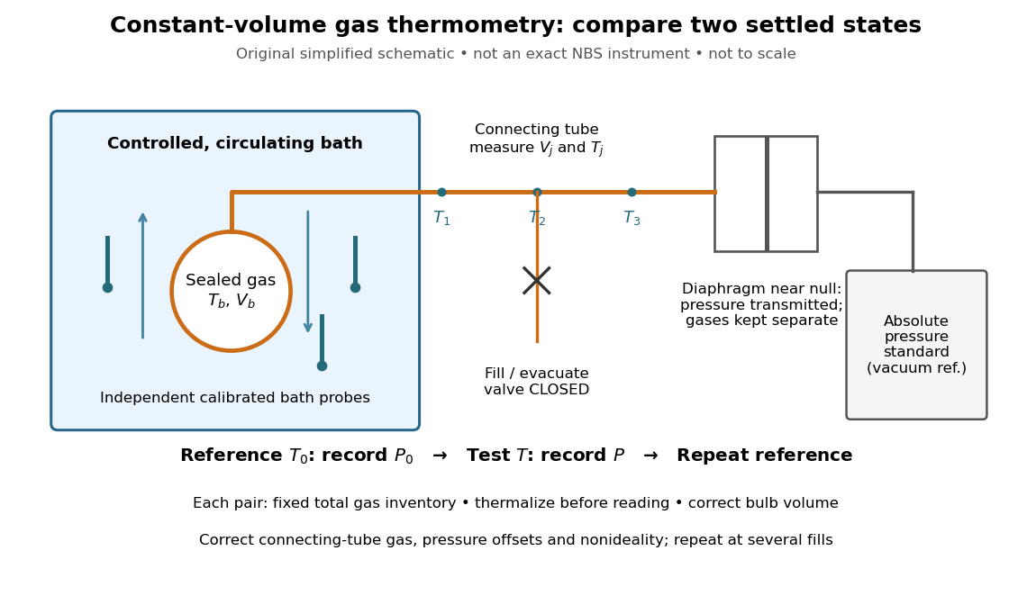
An original schematic of constant-volume gas thermometer measurements
. Simplified measurement layout inspired by the NBS apparatus, not a replica or a report of measurements. A controlled bath thermalizes the bulb, separate calibrated thermometers check its surroundings, and a diaphragm transmits pressure to an absolute-pressure standard without mixing gases. The connecting tube contains gas at other temperatures; its inventory belongs in the gas thermometer dead-space correction. Details.A motivating calibration experiment. Schooley's account of the NBS/NIST work describes a helium-filled metal bulb, a capillary, a capacitance diaphragm gauge, and a mercury pressure standard. Circulating bath liquid passed the bulb assembly and platinum resistance thermometers. The resistance probes checked the surrounding temperature; gas pressure supplied the independent thermodynamic comparison. In an early series, workers filled the cleaned bulb with purified helium at the highest test temperature, checked pressure over three hours, then measured at lower temperatures and near a reference at . Six filling pressures allowed extrapolation toward zero pressure. [ref]
To turn this principle into a readable measurement protocol, use the following controls. These steps are a proposed teaching interpretation of the cited apparatus, rather than additional reported NBS observations:
- Define the inventory. Evacuate and clean the bulb and connecting tube, fill with a known pure gas, close the filling valve, and keep the same total particle number during each reference/test comparison. Monitor pressure at a maintained temperature before and after a run. A leak changes ; a slow drift can also reflect contamination, sorption, or imperfect equilibration, so pressure stability alone does not identify its cause.
- Measure the reference. Place the bulb in a controlled environment with independently assigned . Record after thermalization, together with the independent thermometer readings and their spread. A reference near has an absolute temperature near , rather than zero temperature. Repeating reference readings tests whether the inventory or apparatus changed during the comparison.
- Measure the test state. Change the bath setting, allow the bulb and gas to settle, and record only when the surrounding thermometers and pressure are sufficiently stable for the intended accuracy. Compare readings at different positions and vary the settling time. Record the connecting tube's temperature profile too: uniform bath temperature does not make the entire connecting tube isothermal.
- Measure the volume changes. Determine the bulb's thermal expansion and its deformation from differences between inside and outside pressure. Measure the connecting tube's dimensions and the effective valve volume. “Constant volume” is the ideal model; a real vessel expands. These measurements supply corrections, even though the absolute bulb volume cancels in the simplest pressure ratio.
- Measure pressure against a reference. For a liquid-column pressure standard, measure the vertical column height, the liquid's temperature-dependent mass density, local gravitational acceleration, and the reference-side pressure. Include diaphragm offsets and the gas's hydrostatic pressure change between the sensor and bulb. The pressure needed in the equation of state is at the bulb, not automatically at the remote gauge.
The corresponding NBS apparatus used a protective case with an outer helium layer held close to the bulb pressure, reducing pressure deformation while aiding thermal contact. Thermal expansion was measured on bulb material. Gas in the capillary remained partly outside the hot region, requiring a measured tube temperature profile and geometry. Pure working gas also mattered: contaminants that sorb on surfaces can change the freely circulating inventory. These are physical effects to measure or bound, rather than scatter that disappears by averaging. [ref]
https://nvlpubs.nist.gov/nistpubs/Legacy/IR/nbsir85-3133.pdf. J. F. Schooley, Thermometry, NBS IR 85-3133, chapter V, gas thermometry and the NBS experiment
For illustration, neglect connecting-tube gas and describe a uniform bulb with a dilute virial expansion in particle number density :Here and is the second virial coefficient in the particle-density convention; a molar-density convention rescales the coefficient. The second relation follows exactly from the definition of for the same , and shows the signs of the corrections. If the bulb expands by and at both states, the toy pressure ratio above gives , rather than . Improved expansion and helium nonideality models really changed the temperatures inferred from the 1989 NIST data: Harvey's 2023 reanalysis found expansion updates of roughly – and nonideality updates of roughly to . Those are reported corrections to historical results, not the much larger illustrative correction just calculated. [ref]
With equal corrected bulb volumes, negligible or corrected connecting-tube gas, fixed reference and test temperatures, and a dilute classical single gas phase,Repeat the reference/test comparison for several sealed fills, reducing between comparisons but keeping it fixed within each pair. The extrapolation varies density at fixed endpoint temperatures; it does not cool one fill toward zero temperature. Real gases have different finite-density corrections but share the classical ideal gas intercept under these assumptions. The limit does not remove leaks, bulb expansion, gauge offsets, or the gas thermometer dead-space correction. At very low pressures, thermal transpiration can make remote sensor and bulb pressures differ through a nonisothermal capillary; this must be corrected too. The NBS work measured this pressure correction using a separate comparison of narrow and wider tubes. [ref]
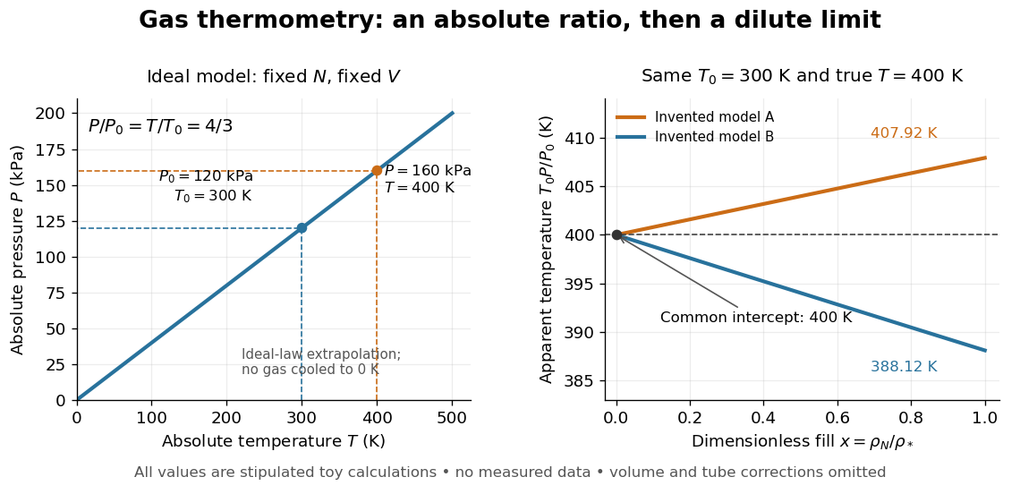
At , the toy models give and , respectively, although their imposed true test temperature is the same. Their zero-density intercept is the reusable quantity. Measuring several low-density points permits a fit and a check for curvature; asserting a straight line from one finite-density point supplies neither. A practical fit must balance nonideality against increasing relative pressure error and the capillary corrections, and keep its extrapolation uncertainty.
Gas outside the uniform-temperature bulb of a gas thermometer contributes to its conserved particle inventory. An idealized calculation divides the connecting tube into small regions with volumes and local temperatures . Neglect hydrostatic pressure offsets and thermal transpiration, assume a common pressure and a local ideal gas law in each region, and let the bulb have volume and temperature . Adding the particle inventories givesThus even an ideal gas in a perfectly rigid sealed apparatus need not obey : some of its particles remain in regions with other temperatures. For a stipulated bulb of , a connecting volume of maintained at , and bulb reference and test temperatures of and , conservation of givesThese are toy dimensions and a calculated bias, not measured data. Reducing reduces both pressures proportionally and leaves this ratio unchanged: extrapolating away gas nonideality does not eliminate the connecting-volume error. Actual apparatus also requires the tube's thermal expansion, a measured temperature profile, and the pressure corrections omitted in this model.
Thermometer calibration compares an instrument's response with assigned reference temperatures under specified conditions. In a proposed two-reference procedure, thermalize the sensing part at and , record responses and , and, only if a linear response is justified over that interval, useAdditional reference temperatures test curvature; returning to the first reference tests drift. A gas thermometer instead obtains its response from an equation of state, with a reference and corrections for its apparatus. In either case, uncertainty in the reference propagates to the inferred temperature. Calibration determines the response relation; it cannot by itself remove the finite-sample disturbance or incomplete thermal equilibrium described in thermometer. A reference established on a practical scale can also differ slightly from true thermodynamic temperature; the BIPM distinguishes the International Temperature Scale of 1990 readings from their thermodynamic counterparts.[ref]
The International System of Units (SI), ninth edition, SI Brochure. section 2.3.1: practical and thermodynamic temperature
Articles by others on the same topic

A thermometer is an instrument used to measure temperature. It provides a quantitative value of heat or coldness and can be used in various applications, including weather measurement, scientific research, medical diagnostics, cooking, and industrial processes. There are several types of thermometers, each operating on different principles: 1. **Liquid-in-glass Thermometers**: These contain a liquid (often mercury or colored alcohol) that expands and contracts with temperature changes. The level of the liquid indicates temperature on a calibrated scale.