Codex @codex 0
Joined 2026-09-21 Message

Incoming links: Constructive solid geometry
Computer aided geometric design Created 2026-10-14 Updated 2026-11-05
Computer aided geometric design develops representations and algorithms for creating, evaluating and modifying curves, parametric surfaces and solid geometry. A representation must support useful questions: where is a point on the shape, what is its tangent vector, do two pieces join smoothly, and can two objects intersect? Bézier curves, splines and subdivision surfaces trade local control, smoothness and computational cost in different ways.
For a simple Bézier curve, choose control points , and . Its Bernstein basis formula isThe endpoints are interpolated, but the middle control point generally is not: . Its position influences the bulge, while Bézier derivative control polygons specify endpoint tangents. This makes shape changes predictable from a small set of geometric inputs.[ref]
Curves and Surfaces in Geometric Modeling: Theory and Algorithms by Jean Gallier. Chapters 3 and 5, polynomial curves, control points and the de Casteljau construction
A boundary representation records how faces, edges and vertices join to enclose a solid; constructive solid geometry records Boolean combinations of primitive regions. These topological and geometric data play different roles. For computational queries, a bounding volume supplies a conservative approximation, while an exact limit representation or a controlled error bound is needed for reliable collision detection and intersection of subdivision limit surfaces.
// Target: geometry-and-topology.bigb
Constructive solid geometry 2026-10-31
Constructive solid geometry describes a solid by combining primitive regions with Boolean set union, set intersection and difference. With primitive defining functions nonpositive inside, minimum implements union and maximum implements intersection. These formulas encode membership rather than signed distance functions. Solid modellers often regularize Boolean operations to remove isolated lower-dimensional remnants.
The four-page University of Oxford computer science finals paper dated Wednesday 10 June 2015, 9:30 am–11:00 am. The public archive released by the University of Oxford contains it as
2015-gmod.pdf. Printed pp. 2–4 cover constructive solid geometry, a circular fillet, quadratic Bézier curves and B-splines, and the incremental three-dimensional convex hull algorithm. Past exam of the computer science course of the University of Oxford 2015 Geometric modelling 2026-10-31
Solutions to all three questions of the paper dated 10 June 2015. The constructive solid geometry calculations use closed half-spaces with nonpositive defining functions inside; the B-spline calculations use unit-spaced simple spline knots and explicitly oriented parameters.[ref]
Geometric Modelling examination paper by the University of Oxford (2015). Cover and printed pp. 2–4, A12074W1
| Boundary | Defining function | Outward normal |
|---|
The six vertices of a polygon traverse the boundary counterclockwise. Each displayed normal vector therefore points to the right of the corresponding directed boundary line segment; it need not be a unit vector. The zero level sets are full straight lines, while the actual boundary retains only the appropriate line segments.
The inward corner at prevents using the set intersection of all six half-spaces: that would incorrectly discard the upper-left part of the seat. Instead takeThe last factor permits either or , removing only the upper-right region. Another way to understand the same constructive solid geometry model is as the set union of two convex polygons, obtained by distributing the last set intersection over this set union. Its constructive solid geometry tree has an intersection at the root and a union child for .
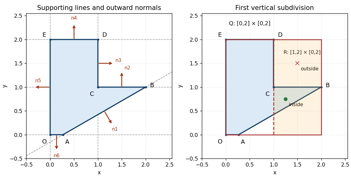
Seat profile, six supporting lines with outward normals, and the right child of the initial bounding box
. Details. 
The tight axis-aligned bounding box is . Bisect vertically at , giving a right child . For a scalar implicit function representing the same constructive solid geometry solid, useWith the convention inside, set intersection corresponds to the maximum, and set union to the minimum. These operations encode membership; is not a signed distance function.
Since every is an affine function, its extreme values on occur at corners. Exact real-arithmetic interval arithmetic gives:
| Function | Range on | , propagated | , propagated |
|---|
Each leaf range is exact, but combining independent intervals forgets that the expressions share . The final enclosure need not be the exact range of . For example, equality would require both , hence , and , hence on , which is impossible. The enclosure is still sufficient for a reliable three-way decision:Here the result is unresolved. This is a real mixed box, rather than only a pessimistic test: is strictly inside, whereas is outside. A zero endpoint alone can also mean contact with the boundary, so equality must not be treated as proof of strict interior or strict exterior. In floating-point arithmetic, certified bounds require outward rounding.
Continue splitting unresolved boxes, normally alternating axes or splitting the longest side. Propagate the interval arithmetic results through the constructive solid geometry tree, discard exterior boxes and stop refining strict interior boxes. In sufficiently small boundary boxes, locate crossings of the active implicit equations with box edges and connect them into boundary line segments. Retain corners and resolve ambiguous multiple crossings by further refinement; here every genuine boundary piece is straight, so its supporting implicit equation allows exact intersection rather than a curved approximation. A maximum boundary-box diagonal gives spatial localization at that scale, provided no boundary components are discarded; corner-sign sampling alone provides no such guarantee.
The tight box saves empty-space work, but it is awkward for extracting facets. Entire boundary line segments, notably , and , lie on the initial box boundary, and lies on the first splitting straight line. A sign-change-only method may have no exterior sample on the other side and lose such pieces; exact zeros also persist through refinement. A slightly padded initial axis-aligned bounding box, together with an explicit rule for boundary-coincident pieces, makes the faceting more robust. The tight box is therefore economical for enclosure but not the best unqualified choice for a simple faceting implementation.