Solutions to all three questions of the paper dated 10 June 2015. The constructive solid geometry calculations use closed half-spaces with nonpositive defining functions inside; the B-spline calculations use unit-spaced simple spline knots and explicitly oriented parameters.[ref]
Geometric Modelling examination paper by the University of Oxford (2015). Cover and printed pp. 2–4, A12074W1
Set and . A displacement from lies along the straight line precisely when its two-dimensional determinant with vanishes. Thus an implicit equation isEquivalently, write , with , and . The vector is a normal vector. The formula handles vertical and horizontal straight lines without division. It presupposes : coincident points do not determine a unique straight line.
Solving the implicit equation for when givesHere “gradient” means the slope , rather than the gradient of an implicit defining function. If and , the straight line is vertical and has no finite slope. If and , its slope is zero.
For , substitute or , respectively:In terms of the original coordinates, these arewith each expression used only when its denominator is nonzero. If , the straight line is horizontal: it misses the horizontal axis unless , in which case it is that entire axis. If , it is vertical: it misses the vertical axis unless , in which case it is that entire axis. A straight line through the origin has both finite intercepts equal to the origin whenever neither axis is coincident with it.
| Boundary | Defining function | Outward normal |
|---|
The six vertices of a polygon traverse the boundary counterclockwise. Each displayed normal vector therefore points to the right of the corresponding directed boundary line segment; it need not be a unit vector. The zero level sets are full straight lines, while the actual boundary retains only the appropriate line segments.
The inward corner at prevents using the set intersection of all six half-spaces: that would incorrectly discard the upper-left part of the seat. Instead takeThe last factor permits either or , removing only the upper-right region. Another way to understand the same constructive solid geometry model is as the set union of two convex polygons, obtained by distributing the last set intersection over this set union. Its constructive solid geometry tree has an intersection at the root and a union child for .
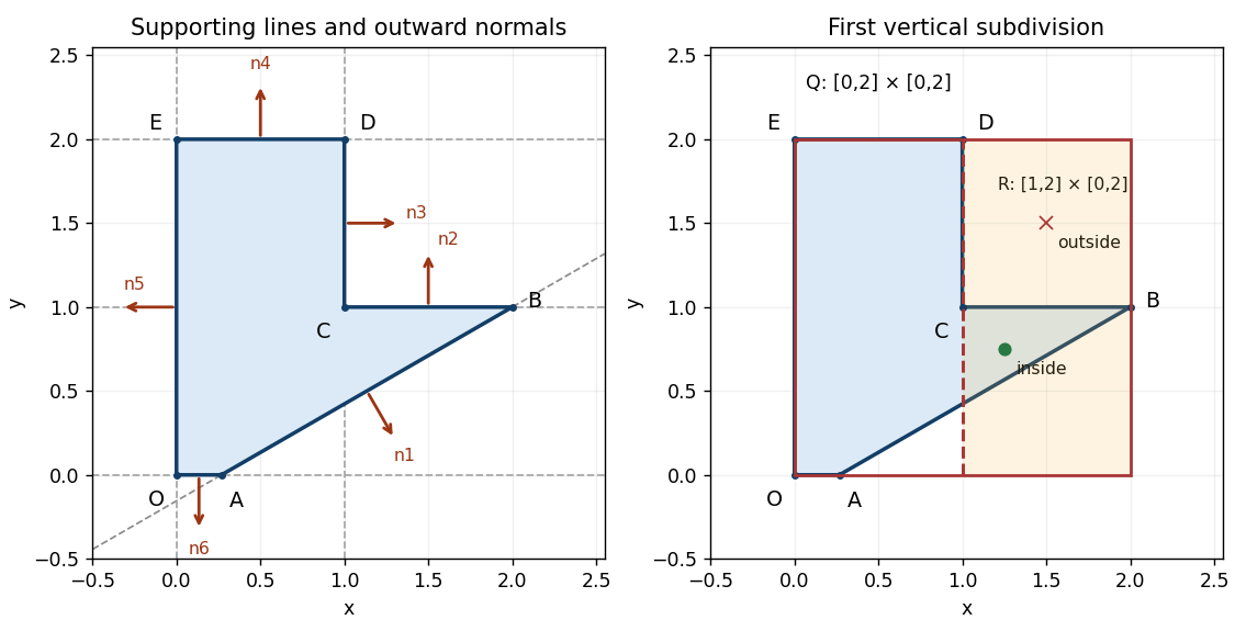
Seat profile, six supporting lines with outward normals, and the right child of the initial bounding box
. Details. The tight axis-aligned bounding box is . Bisect vertically at , giving a right child . For a scalar implicit function representing the same constructive solid geometry solid, useWith the convention inside, set intersection corresponds to the maximum, and set union to the minimum. These operations encode membership; is not a signed distance function.
Since every is an affine function, its extreme values on occur at corners. Exact real-arithmetic interval arithmetic gives:
| Function | Range on | , propagated | , propagated |
|---|
Each leaf range is exact, but combining independent intervals forgets that the expressions share . The final enclosure need not be the exact range of . For example, equality would require both , hence , and , hence on , which is impossible. The enclosure is still sufficient for a reliable three-way decision:Here the result is unresolved. This is a real mixed box, rather than only a pessimistic test: is strictly inside, whereas is outside. A zero endpoint alone can also mean contact with the boundary, so equality must not be treated as proof of strict interior or strict exterior. In floating-point arithmetic, certified bounds require outward rounding.
Continue splitting unresolved boxes, normally alternating axes or splitting the longest side. Propagate the interval arithmetic results through the constructive solid geometry tree, discard exterior boxes and stop refining strict interior boxes. In sufficiently small boundary boxes, locate crossings of the active implicit equations with box edges and connect them into boundary line segments. Retain corners and resolve ambiguous multiple crossings by further refinement; here every genuine boundary piece is straight, so its supporting implicit equation allows exact intersection rather than a curved approximation. A maximum boundary-box diagonal gives spatial localization at that scale, provided no boundary components are discarded; corner-sign sampling alone provides no such guarantee.
The tight box saves empty-space work, but it is awkward for extracting facets. Entire boundary line segments, notably , and , lie on the initial box boundary, and lies on the first splitting straight line. A sign-change-only method may have no exterior sample on the other side and lose such pieces; exact zeros also persist through refinement. A slightly padded initial axis-aligned bounding box, together with an explicit rule for boundary-coincident pieces, makes the faceting more robust. The tight box is therefore economical for enclosure but not the best unqualified choice for a simple faceting implementation.
Choose a circular fillet that removes the sharp convex tip at . The unit directions from toward and are and . Therefore the prescribed tangent points areThe circle centre lies on the normal line to through , so . Its radius to must be perpendicular to , whose direction vector is . ThusConsequentlyIndeed . The interior angle is , and the same radius follows from . The selected circular arc runs from to through angles around :The circular arc facing is the rounding; the complementary arc is not part of the boundary.
Define the disk and a half-plane through the chord byBoth satisfy , and . The clipping half-space retains the part away from , while the disk restores the rounded cap. The required local constructive solid geometry tree isOnly the portion of on the side of can be removed. To see the locality, is negative at every original vertex of a polygon except , and vanishes on the two adjacent sides exactly at . In the resulting triangle , the disk keeps the curved cap next to and discards the tip at . A global set intersection with alone would destroy most of the seat. The outward normal vector on the new boundary is ; at it has the same direction as the outward normal vectors of .
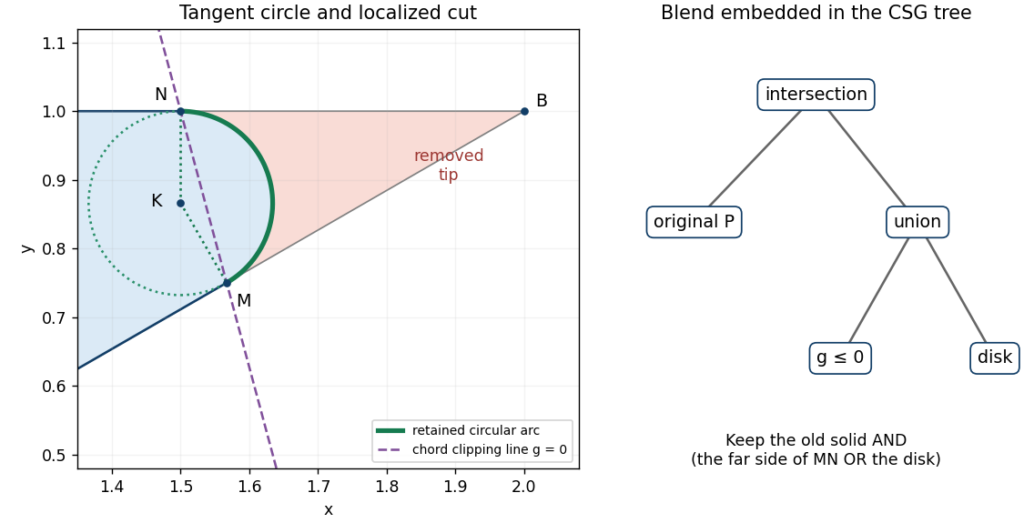


The tangent constraints alone do not insist on a circle; other conic sections can give different bulges. For example, a positive-weight rational quadratic Bézier curve with handles has the required tangent directions:Varying changes the bulge while fixing the tangent points; the circular choice has . Once a circular fillet and these two tangent points are chosen, its centre and radius have no remaining freedom. The half-plane sign and arc selection are also essential: reversing them chooses a different retained region. This construction gives matching tangent directions, or first-order geometric continuity, at ; the curvature jumps from zero on each straight side to on the circle.
Insert the union subtree from part (f) as another child of the original intersection:Thus the constructive solid geometry tree has one intersection root, four original half-space leaves and two union children. The first union handles the inward corner at ; the second embeds the circular fillet at . The line segments and now end at and start at , with the chosen circular arc between them. All other boundary line segments are retained.
For a fixed , De Casteljau's algorithm first takes the same fractional position along both adjacent sides of the control polygon:It then applies another linear interpolation with that same :This is the degree-two Bernstein basis representation of a quadratic Bézier curve. Its coordinate polynomials areThe degree is exactly two, since its second derivative is nonzero. As a check on the construction, at the two intermediate points are and and their midpoint is .
Three useful geometric properties, with their concrete consequences here, are:
- Endpoint interpolation. and . The middle control point is a handle, not an interpolated point: , so the curve never reaches .
- Endpoint tangents. and . Thus the tangent lines are parallel to the first and last sides of the control polygon, respectively; both endpoint derivatives are nonzero.
- Convex-hull containment. The three Bernstein basis weights are nonnegative and sum to one on . Every is therefore a convex combination of , so the entire Bézier curve lies in their filled triangle.
These give the compact answerThe same sum-to-one calculation also explains affine equivariance of a geometric basis: applying an affine map to the handles applies that map to the curve.
Use a row of descending monomials and a matrix with one control point per row. Expanding gives their coefficients in the three columns of the basis matrix:The matrix multiplication isIn particular, , so multiplying the geometric matrix takes exactly the weighted control point sum in part (a). The two output entries are . The basis matrix depends only on the degree and ordering convention; holds the particular geometry.
Choose a quadratic uniform B-spline segment on a unit spline knot interval. This choice is useful because adjacent pieces can later share de Boor points at simple, equally spaced spline knots. Its three active basis pieces on local areThey follow from the Cox-de Boor recurrence for degree two and consecutive integer spline knots. If the three de Boor points are , then the equivalent Bézier curve handles areOne can verify this conversion simply by substituting these expressions into the Bernstein basis formula and collecting each . Solving givesThe desired matrix representation is thereforeThe left row is again the monomial row, the middle matrix contains the monomial coefficients of , and the right matrix lists the de Boor points. Unlike the Bézier curve basis matrix, the constant row averages two handles. A clamped B-spline with repeated end spline knots could instead reuse directly; the simple uniform convention above specifies which representation is being used and supplies the shared handles required for the extension.
Rotating the geometry through sends every point to . To start the extension at the origin, also reverse the parameter:Then and . Merely using would trace the same rotated image toward the origin, instead of away from the join.
The reversed and rotated de Boor points are , namely . The first two are already , so there is only one new de Boor point, . Using the same uniform basis matrix,Equivalently, the Bézier curve handles are , and , which gives the same polynomials immediately.
Assign one unit parameter interval to each piece. ThenThere is no ambiguity at , since both pieces give the origin. For a single B-spline representation take degree two, the four de Boor pointsand the equally spaced spline knot vector . With denoting the normalized degree-two B-spline on this vector, the complete valid parameter interval is andOn the active handles are , and on they are . Shared handles and a simple interior spline knot are what merge the two pieces into one uniform B-spline. The exterior spline knots support the basis; they do not extend the interval being drawn.
In particular, the requested horizontal pieces and their vertical counterparts are
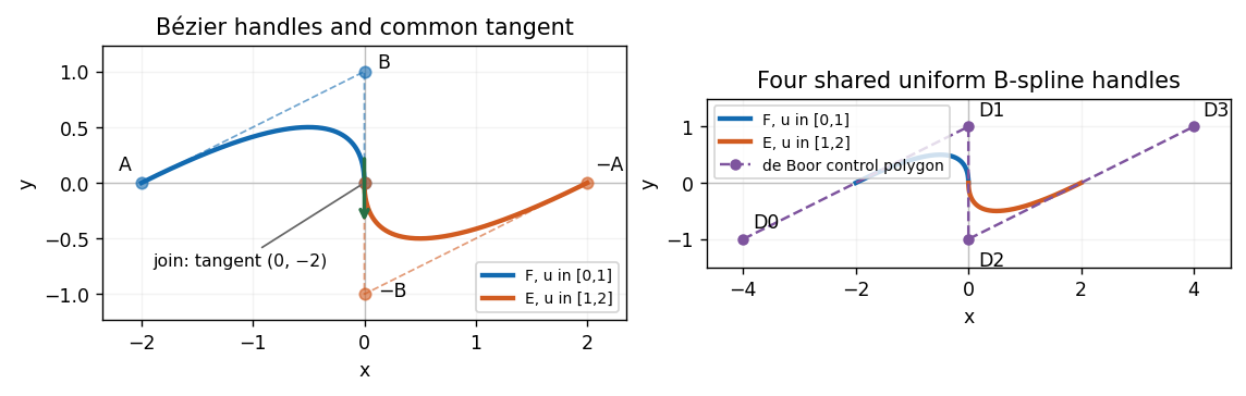
Two quadratic pieces, their Bézier handles, the shared uniform B-spline control polygon, and the vertical tangent at the join
. Details. 
The join has matching positions and first derivatives:Because both pieces have unit parameter intervals, these are also the one-sided derivatives of at . Thus has first-order parametric continuity, and hence first-order geometric continuity, with no corner or cusp. Its nonzero tangent vector points vertically downward.
The second derivatives do not agree:So this is but not parametric continuity. The signed planar curvature has one-sided valuesThe unsigned curvatures agree, but the bending switches sides; there is no second-order geometric continuity through a regular orientation-preserving reparametrization. The join is a reversal of bending with a curvature jump, rather than a smooth zero-curvature inflection.
For the “gradient” compute away from the join:HenceThe zero horizontal derivative is not a stationary point of the parametric curve, since its vertical derivative is . It means that the locally regular curve has a vertical tangent line and cannot have a finite graph derivative as there.
For solid modelling, a polyhedron is a solid whose boundary consists of finitely many planar polygons, called faces, meeting along straight edges and at vertices of a polyhedron. A face is not merely a list of arbitrary spatial points: its boundary must lie in one plane and bound a valid planar region. The boundary is closed and consistently oriented so that inside and outside are defined.
For example, a tetrahedron has four triangular faces, six edges and four vertices of a polyhedron. A more general polyhedron need not be convex and can have handles or cavities. The concise definition is
For an ordinary closed manifold boundary representation, three requirements are:
- Valid embedded faces. Each face is planar and bounded by simple closed edge loops with nonzero area; distinct face interiors do not cross, and faces meet only in their declared common edges or vertices of a polyhedron. A quadrilateral with four noncoplanar vertices of a polyhedron is not one planar face; a bow-tie loop does not bound a simple face. Holes, when allowed, need separate correctly oriented loops.
- Closed manifold incidence. Exactly two faces meet at each edge, and the incident faces around each vertex of a polyhedron form one cyclic fan. A single missing face leaves edges incident with only one face. Three faces sharing an edge, or two closed shells touching only at one vertex of a polyhedron, violate the local surface condition. The second example shows why the edge count alone is insufficient.
- Consistent orientation. Adjacent oriented faces traverse their common edge in opposite directions, giving compatible outward normal vectors. Reversing just one face of a tetrahedron breaks this condition. For a cavity, the material's outward normal vector points into the cavity, so shell orientation must also respect which region is solid.
Together these support the answerFor a connected orientable closed boundary of genus , the Euler characteristic provides an additional check, , when faces are disk-like. The familiar value applies to a sphere-like shell; it must not be imposed blindly on every polyhedron. Correct counts alone do not exclude intersections or invalid local incidence.
A boundary representation separates geometry, which supplies locations and supporting planes, from topology, which specifies incidence and orientation. A practical winged-edge data structure uses three related record types:
- A vertex of a polyhedron record holds its three coordinates and a reference to one incident edge, sufficient to begin traversing the local fan.
- A face record holds its supporting plane, an outward normal vector or equivalent orientation, and a reference to a boundary edge. Faces with holes need one entry per boundary loop.
- An edge record holds its two endpoint vertices of a polyhedron, its left and right incident faces, and predecessor and successor edges around each of those faces: four “wing” references. “Left” and “right” refer to a chosen orientation of the edge and compatible face traversal conventions.
This explicitly stores adjacency rather than recovering it by searching all faces. A half-edge data structure expresses much the same information with two oppositely directed records per undirected edge: each has an origin vertex of a polyhedron, an incident face, its next boundary record and its opposite record; a previous record is often stored as well. The destination can be obtained from the opposite record's origin. This mesh record is distinct from a dangling half-edge of a graph.
The compact implementation answer isThere is deliberate redundancy: the same adjacency can be reached from both an edge and a face, a stored previous edge is recoverable by walking the loop, and a face normal vector can be computed from its ordered noncollinear vertices of a polyhedron. These copies make neighbourhood queries and local edits cheap, and cached plane equations speed geometric tests. They impose consistency obligations: an edit must update reciprocal references, loops, orientations and affected geometric caches together. A half-edge data structure should share the undirected edge's geometry or keep its paired records synchronized.
For a finite nonempty collection , its convex hull is the smallest convex set containing all the points. Equivalently, it is the set of all convex combinations:Every convex set containing the must contain these combinations; the displayed set is itself convex and contains each , proving the equivalence. For a full-dimensional finite collection this is a convex polyhedron. A collinear or coplanar collection instead has a lower-dimensional convex hull, so the solid case needs a separate dimensionality assumption.
Use the straightforward incremental three-dimensional convex hull algorithm. Assume distinct input points, at least four noncoplanar points, and general position with no four coplanar. Use exact orientation decisions, or robust predicates that certify the same signs. These assumptions avoid the separate bookkeeping for flat faces, points on the boundary and lower-dimensional initial data.
- Select four points forming a nondegenerate tetrahedron. Store its four triangular faces with outward normal vectors and consistent adjacency.
- For the next point , evaluate every current oriented face usingThe current hull lies in . Thus a face is visible from exactly when .
- If no face is visible, discard : it lies in the current convex hull. Otherwise identify the horizon of a convex polyhedron seen from , namely the edges incident with exactly one visible and one retained face.
- Delete the visible faces and cone the ordered horizon of a convex polyhedron to , adding one triangle per horizon edge. Orient each new face consistently outward and continue with the next point.
The determinant is six times the oriented volume of the tetrahedron ; only its sign matters. A zero value needs a declared degeneracy policy if the general-position assumption is relaxed.
The data structure update is a separate local operation. Mark visible faces and walk their adjacency to collect the horizon cycle before deleting anything. Remove edges with two visible incident faces; retain horizon edges and their retained-face links. Insert a vertex of a polyhedron record for and a new edge from to each horizon vertex of a polyhedron. Add one face per horizon edge, connect its other two edges to its neighbours in the cone, and replace the deleted face reference on each horizon edge. Restore the cyclic boundary references and each retained vertex of a polyhedron's incident-edge reference; remove any old vertices of a polyhedron left without incident faces.
For an outward visible face with boundary edge on the horizon, the new outward face can be ordered . Its retained neighbour already traverses that edge as . As an independent orientation check, an interior point of the old hull must evaluate negatively against the new face.
The correctness step is geometric: the nonvisible part of a convex polyhedron remains supporting, while sight lines from to the horizon create precisely the new supporting faces. Replacing the visible cap by its cone therefore givesInduction from the initial tetrahedron yields the convex hull of all input points.
With processed points, a triangulated three-dimensional convex hull has faces and edges. For a sphere-like triangular boundary, the Euler characteristic and give and , with . The complete face scan, horizon construction and adjacency update in the implementation of part (e) therefore cost per insertion. Consequently,The quadratic worst case really occurs for this implementation. Choose all input points in strictly convex position, for example distinct points on the three-dimensional moment curve. Each processed point remains a hull vertex of a polyhedron, so the hull has triangular faces after insertions. Scanning every face at every next insertion takes sign tests. This argument does not require every insertion to delete most faces: the repeated global scans already force the bound. More elaborate convex hull algorithms with different search machinery are not the implementation being analysed here.
Insert the points in their given order, starting from . Use outward face orientation and regard as the interior side. The initial tetrahedron is nondegenerate becauseThus its volume is . The following table gives consistently oriented faces, conveniently scaled plane equations, and the omitted old vertex of a polyhedron test:
| Face order | Interior inequality | Value at the opposite vertex |
|---|
Every opposite vertex of a polyhedron is strictly on the interior side, so these orientations are correct. The intersection of these four half-spaces is exactly the initial tetrahedron.
Now test . In the same row order the face expressions giveTherefore and are visible and must be removed; and are retained. The common edge lies inside the deleted patch and is removed. The directed horizon isCone this cycle to , giving outward face orders . Their equations and tests of the two old vertices of a polyhedron not belonging to each face are:
| New face | Interior inequality | Tests of the other vertices |
|---|
Each new plane contains its three named vertices of a polyhedron and has all remaining input points strictly on the interior side. Together with the two retained half-spaces, these six supporting inequalities describe the final convex hull:Equivalently assemble the closed oriented boundary from , with adjacent face loops traversing shared edges in opposite directions. It is a triangular bipyramid with base triangle and apices ; is internal, so it is not a boundary face. There are five vertices of a polyhedron, nine edges and six faces, giving the check . The initial tetrahedron similarly has .
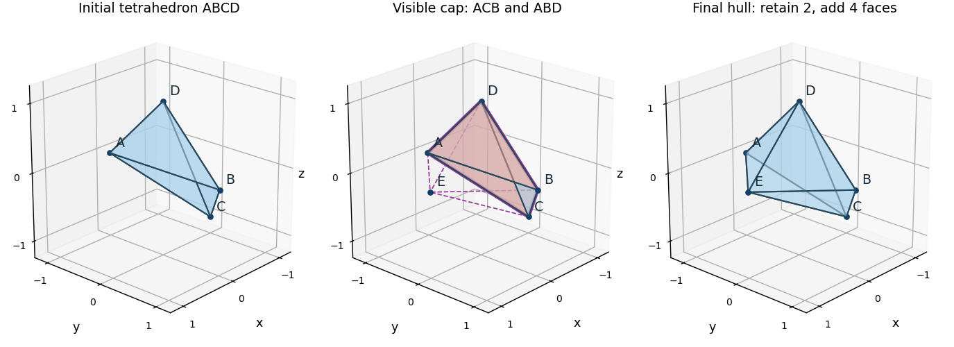
Initial tetrahedron, the two faces visible from E and their horizon, and the final six-face convex hull
. Details. 
Articles by others on the same topic
There are currently no matching articles.