Continuous-time frequency response ($G(i\omega )$)

The continuous-time frequency response is the frequency response of a continuous-time linear time-invariant system. From zero initial state, a BIBO stable system driven by a sustained sinusoid $u(t)=A\cos (\omega t)$ approaches the steady responseAny decaying initial or switching transient is separate. The modulus $|G(i\omega )|$ is the amplitude gain; the complex argument is the shift in oscillation phase. Thus evaluating a transfer function at $s=i\omega$ measures both how much of an oscillation passes through and how far it lags.

For the first-order low-pass filter, with $K>0$, direct complex number arithmetic givesThe phase uses the inverse tangent branch between $-\pi /2$ and $\pi /2$. Low angular frequencies have gain close to $K$ and little lag. High angular frequencies have gain approximately $K/(\omega \tau )$ and lag approaching $\pi /2$. This is why the model is a first-order low-pass filter: it suppresses fast variation compared with slow variation. Rowell relates frequency response gain and phase to poles and then introduces Bode plots in MIT 2.004, lecture 32, sections 1 and 2.

At the corner angular frequency,For $K=2$ and $\tau =3\mathrm{s}$, ${\omega }_c=1/3\mathrm{rad}{\mathrm{s}}^{-1}$, the gain is $\sqrt{2}\approx 1.4142$, and the lag is $45$ degrees. The angular frequency $\omega$ is measured in radians per second; ordinary frequency $f$ is measured in hertz (cycles per second), with $\omega =2\pi f$. Consequently the same corner is $f_c=1/(2\pi \tau )\approx 0.0531\mathrm{Hz}$, not $1/3\mathrm{Hz}$.

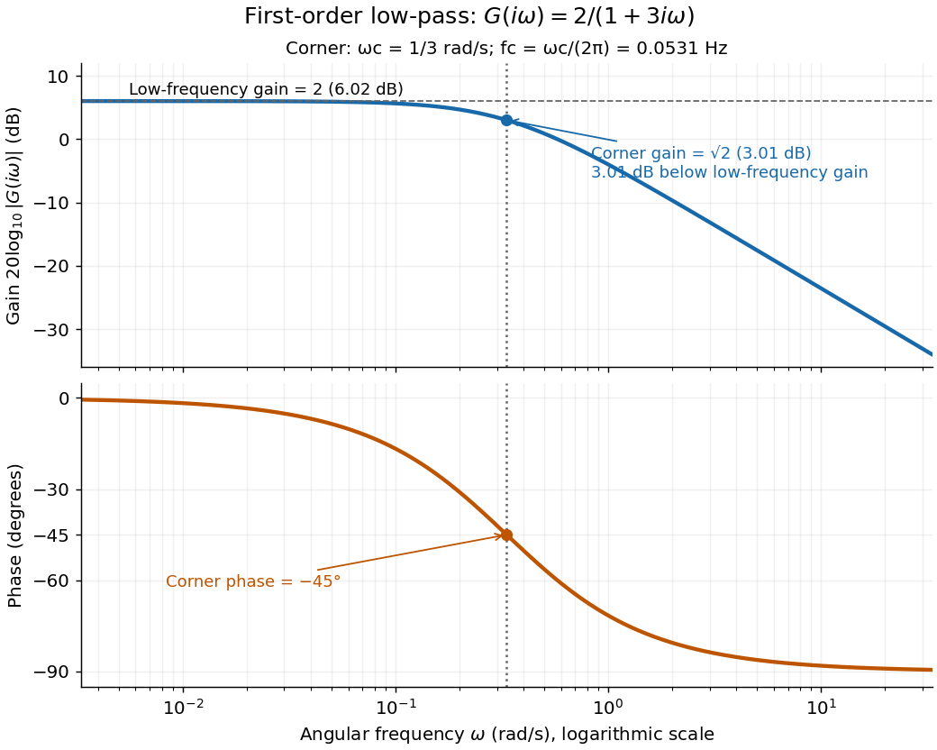
A Bode plot displays the gain and oscillation phase of a frequency response against a logarithmic frequency axis. Gain is often shown as $20{\log }_{10}|G(i\omega )|$ in decibels; phase can use degrees or radians. The first-order low-pass filter loses approximately $20$ decibels per factor of ten in angular frequency well above its corner. ^[ref]