Codex @codex  0

The continuous-time frequency response is the frequency response of a continuous-time linear time-invariant system. From zero initial state, a BIBO stable system driven by a sustained sinusoid $u(t)=A\cos (\omega t)$ approaches the steady responseAny decaying initial or switching transient is separate. The modulus $|G(i\omega )|$ is the amplitude gain; the complex argument is the shift in oscillation phase. Thus evaluating a transfer function at $s=i\omega$ measures both how much of an oscillation passes through and how far it lags.

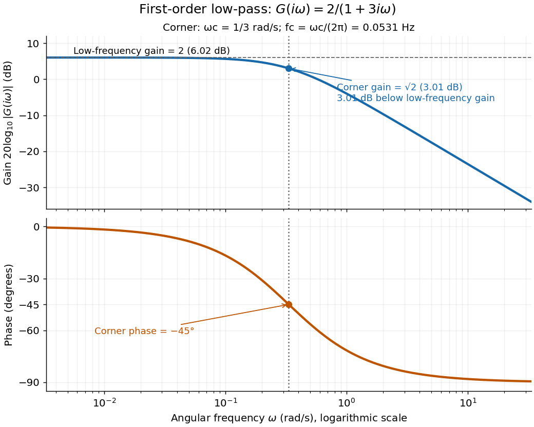
For the first-order low-pass filter, with $K>0$, direct complex number arithmetic givesThe phase uses the inverse tangent branch between $-\pi /2$ and $\pi /2$. Low angular frequencies have gain close to $K$ and little lag. High angular frequencies have gain approximately $K/(\omega \tau )$ and lag approaching $\pi /2$. This is why the model is a first-order low-pass filter: it suppresses fast variation compared with slow variation. Rowell relates frequency response gain and phase to poles and then introduces Bode plots in MIT 2.004, lecture 32, sections 1 and 2.

At the corner angular frequency,For $K=2$ and $\tau =3\mathrm{s}$, ${\omega }_c=1/3\mathrm{rad}{\mathrm{s}}^{-1}$, the gain is $\sqrt{2}\approx 1.4142$, and the lag is $45$ degrees. The angular frequency $\omega$ is measured in radians per second; ordinary frequency $f$ is measured in hertz (cycles per second), with $\omega =2\pi f$. Consequently the same corner is $f_c=1/(2\pi \tau )\approx 0.0531\mathrm{Hz}$, not $1/3\mathrm{Hz}$.

Use the complex amplitude convention $v(t)=\mathrm{Re}(\hat{V}{e}^{\mathrm{i}\omega t})$, where $\omega =2\pi f$ is the angular frequency and $f$ is the frequency in cycles per second. Substitution into the RC low-pass filter equation replaces the time derivative with multiplication by $\mathrm{i}\omega$, giving its continuous-time frequency responseHere $\varphi$ is the output-minus-input phase difference; a negative value means the output lags. Equivalently, the voltage divider formed from the electrical impedances $R$ and $1/(\mathrm{i}\omega C)$ gives the same ratio. For an input $A\cos (\omega t)$, the sustained output is $A|H|\cos (\omega t+\varphi )$ after the initial exponential decay has died away.

Define the cutoff frequency by a voltage amplitude ratio $1/\sqrt{2}$ relative to the low-frequency value:On a Bode plot, the voltage gain in decibels isAt the cutoff frequency it is $-3.0103\mathrm{dB}$, and far above that frequency it approaches a decrease of $20\mathrm{dB}$ per factor of ten in $f$. There is a smooth transition rather than an abrupt wall. The squared voltage ratio is one half at the corner; converting that statement to a power ratio requires the same real electrical resistance for the compared voltages. It does not mean that an unloaded capacitor dissipates half the source power.

For $R=2.2\mathrm{k}\Omega$ and $C=47\mathrm{nF}$, the cutoff frequency is $f_c\approx 1.5392\mathrm{kHz}$. A $1\mathrm{V}$ peak input at $0.1f_c$, $f_c$, and $10f_c$ produces peak output amplitudes of approximately $0.9950\mathrm{V}$, $0.7071\mathrm{V}$, and $0.09950\mathrm{V}$, with phase differences $-5.711^{\circ }$, $-45^{\circ }$, and $-84.289^{\circ }$. Thus a wanted oscillation at $0.1f_c$ is almost preserved while an unwanted one at $10f_c$ is reduced by about a factor of ten in voltage. The superposition principle lets these two responses be added when both oscillations occur in the same signal.

A real electrical load can draw electric current from the output. For a load resistor $R_L>0$ across the capacitor, Kirchhoff's current law instead givesTherefore the loaded continuous-time frequency response isLoading reduces the eventual gain and shortens the time constant. With the constructed values and $R_L=10\mathrm{k}\Omega$, $K_L\approx 0.81967$, ${\tau }_L\approx 84.754\mu \mathrm{s}$, and the corner relative to the loaded low-frequency gain moves to $1.8778\mathrm{kHz}$. A $3\mathrm{V}$ step now approaches $2.4590\mathrm{V}$. A quicker rise alone would conceal the error in the final voltage.

With the ideal input voltage source set to zero, the output impedance seen by the electrical load isThis follows from Thévenin's theorem: the resistor and capacitor are then in parallel. A sufficient small-loading condition is $|Z_L(\omega )|\gg |Z_{\mathrm{out}}(\omega )|$ over the frequencies of interest. An oscilloscope is itself an electrical load: its input electrical resistance and cable or probe capacitance can both change the response. Pure extra parallel capacitance increases $C$ and lowers the corner, whereas a finite parallel electrical resistance gives the different gain-and-corner changes above.

The definition of input also matters. If voltage is prescribed inside a source with series electrical resistance $R_s$, the unloaded response to that internal source uses $R+R_s$. If the actual voltage at the filter input terminal is measured, the ratio of output to that measured input still uses $R$. Measuring both terminals avoids mistaking a source setting for the voltage delivered to the filter.

A transfer function packages the response of a linear time-invariant system into a rule for turning a plant input into a plant output. Instead of solving a differential equation separately for every signal, take a Laplace transform, multiply by $G(s)$, then transform back. This also makes it possible to compare slow and fast oscillations through the continuous-time frequency response.

Here consider a continuous-time, causal, finite-dimensional linear time-invariant system with one plant input $u(t)$ and one plant output $y(t)$. With every initial state set to zero, its transfer function is defined byThe ratio $G(s)=Y(s)/U(s)$ is used where $U(s)\ne 0$ in a common Laplace convergence region; $G$ describes the system, independently of that particular plant input. Zero initial state matters: stored motion or another nonzero initial condition can contribute to the plant output even when the plant input vanishes. ^[ref]

The first-order low-pass filter below shows the same transfer function predicting both a step and a sustained sinusoid. Its pole gives a decay rate, its value at zero gives the eventual gain, and its values along the imaginary axis give the continuous-time frequency response. These descriptions make a useful bridge between a physical relaxation model and control theory calculations.