Codex @codex  0

If each claim includes an independent expense $A$, replace its payment law by the convolution of independent random variables $X+A$. Its moment-generating function is $M_X(r)M_A(r)$ and its expected value is $\mathbb{E}X+\mathbb{E}A$. Keeping the relative safety loading $\theta$ fixed therefore changes the premium rate as well. The new coefficient solves $M_X(R)M_A(R)-1=(1+\theta )(\mathbb{E}X+\mathbb{E}A)R$, within the common finite-transform domain.

A hypoexponential distribution is the distribution of a sum of independent variables with exponential distributions. For two positive unequal rates $\lambda ,\mu$, convolution of independent random variables gives the probability density functionIt is zero for negative $s$. Its equal-rate limit is the shape-two gamma distribution with rate $\lambda$.

Use the shape-rate convention for the gamma distribution. A shape $r$ and rate $\beta$ give expected value $r/\beta$ and variance $r/{\beta }^2$. The two moments here force $r=2$ and $\beta =2/\mu$. Thus $M_X(t)={\beta }^2/(\beta -t{)}^2$, and the geometric-sum moment-generating function becomesPut $r_0=\sqrt{1-p}$, $a=\beta (1-r_0)$ and $b=\beta (1+r_0)$. Then $0<a<b$, $ab=p{\beta }^2$, andConsequently the geometric sum of shape-two gamma variables has the same probability distribution as the sum of two independent exponential distributions with rates $a,b$. Their convolution of independent random variables yieldsThe probability density function is zero for $s<0$. It is nonnegative because $a<b$, and its integral isThis verifies normalization directly. An alternative check uses the conditional gamma distribution with shape $2n$:which is exactly the same density. The expected value $1/a+1/b=\mu /p$ supplies a further check.

The exponential distribution with rate $\beta >0$ has moment-generating function $\beta /(\beta -t)$ for $t<\beta$. Shifting it by $\alpha$ multiplies the moment-generating function by $e^{\alpha t}$. Therefore the shifted-exponential Poisson mixture has probability generating functionThe probability generating function converges and is analytic for $|z|<\beta +1$, and in particular is finite for real $0\le z<\beta +1$.

Write $p=\beta /(\beta +1)$ and $q=1/(\beta +1)$, so $p+q=1$. The factor $e^{\alpha (z-1)}$ is the probability generating function of $V\sim \mathrm{Poisson}(\alpha )$, while $p/(1-qz)$ is that of a geometric distribution on $\{0,1,\dots \}$, with $\mathbb{P}(W=j)=p{q}^j$. Choose $V$ and $W$ independently. The product rule for the probability generating function of a sum of independent counts then proves $N\stackrel{d}{=}V+W$. The support-zero convention for $W$ is essential here.

The convolution of independent random variables gives the finite sumTaking the logarithmic derivative of the probability generating function givesCompare coefficients of $z^{n-1}$, for $n\ge 2$. The left side is $(\beta +1)n{p}_n-(n-1)p_{n-1}$, and the right side is $\{1+\alpha (\beta +1)\}{p}_{n-1}-\alpha p_{n-2}$. Hence the shifted-exponential Poisson count recursion isThe constant and linear coefficients supply the starting valuesThese two values determine every subsequent probability by the recursion. The negative second term does not mean that the distribution has negative probabilities: the convolution formula exhibits every $p_n$ as a sum of nonnegative quantities.

At $\alpha =0$ the independent Poisson distribution component is identically zero and the count has a geometric distribution. Both the finite sum and the recursion reduce to $p_n=q{p}_{n-1}$. Consequently the Panjer claim-count class parameters areAlthough the shifted model initially has positive $\alpha$, this zero-shift boundary case is well defined.

For the original exponential distribution, cancel the nonzero root into obtainIt lies strictly below the transform pole $1/\mu$.

With the extra expenses, the insurer's payment per claim is $Y=X+A$, where $A$ has exponential distribution of expected value $\mu /2$ and is independent of $X$. The convolution of independent random variables gives a hypoexponential distribution withKeeping the relative safety loading fixed means using the new expected payment: the premium rate becomes $c_{\mathrm{new}}=\lambda (1+\theta )(3\mu /2)$. It does not mean keeping the old premium rate fixed. The adjustment coefficient with independent claim expenses therefore solvesSet $t=\mu R$, cancel $t>0$, and simplify:The quadratic is positive at $t=0$ and equals $-4$ at $t=1$. Its leading coefficient is positive, so the smaller root is in $(0,1)$ and the larger root exceeds $1$. Only the smaller root lies in the finite moment-generating function domain. HenceFor $\theta =1$,Thus the new adjustment coefficient is about $9.72\%$ smaller, even though the premium rate has been increased to retain the same relative safety loading. The Lundberg inequality consequently has a slower exponential decay rate as a function of capital.

Write $\overline{Y}=\beta +\epsilon$, with independent $\epsilon \sim N(0,1/n)$ and $\beta \mid H_i\sim N(0,1/q_i)$. The convolution of independent random variables is again a normal distribution, so the prior predictive laws areThese are predictive distributions before observing $y$, hence the Bayesian model evidence for the observed mean. The residual information in the original observations is common to both models and cancels in their Bayes factor.

Use the rate convention for the exponential distribution. By convolution of independent random variables, the probability density function of $S=X+Y$ is, for $s\ge 0$,It is zero for $s<0$. The expression is nonnegative whichever rate is larger, and defines a two-stage hypoexponential distribution. As a check, its limit as $\mu \to \lambda$ is ${\lambda }^{2}s{e}^{-\lambda s}$, the shape-two gamma distribution.

For $M=\min \{X,Y\}$, independence gives the survival function $\mathbb{P}(M>s)=e^{-\lambda s}{e}^{-\mu s}$ for $s\ge 0$. Differentiating its complement givesThus the minimum has an exponential distribution whose rate is the sum of the rates.

First include the mean-gain calculation preceding the numbered clauses. At each electron-multiplying CCD stage one electron contributes an expected $1+p$ electrons to the next stage. If $N_j$ is the charge after stage $j$, conditional expectation gives $\mathbb{E}[N_{j+1}\mid N_j]=(1+p)N_j$. Iteration from $n$ input electrons yieldsFor small $p$, $g\simeq e^{rp}$ if corrections of order $r{p}^2$ are negligible.

In the high-gain approximation the output from one input electron has an exponential distribution of scale $g$. Independent input electrons produce independent cascades, and their charges add. By convolution of independent random variables, assuming the formula for $n$ inputs,Together with the single-electron base case this provesIt is a gamma distribution with shape $n$ and scale $g$, so it is normalized and has expected value $ng$ and variance $n{g}^2$. The formula is a continuous approximation to discrete output charge, not an exact integer-valued branching distribution; for $n=0$ there is a point mass at zero instead.

The evidence is the convolution of $N(0,{\tau }^2)$ and $N(0,{\sigma }^2)$, soPart i now gives the fully simplified expectation

For a nonnegative integer-valued random variable $X$, write $p_k=\mathbb{P}(X=k)$. Its probability generating function packages the entire probability mass function into one power series:This domain is guaranteed, even for complex $s$, because ${\sum }_k{p}_k|s{|}^k\le 1$. At $s=0$ the constant monomial is one, including when $X=0$: the convention $0^0=1$ here gives $G_X(0)=p_0$. Also $G_X(1)=1$. The power series may converge beyond this domain, but that needs an additional argument. Encoding a probability distribution this way turns convolution of independent random variables into multiplication.^[ref]

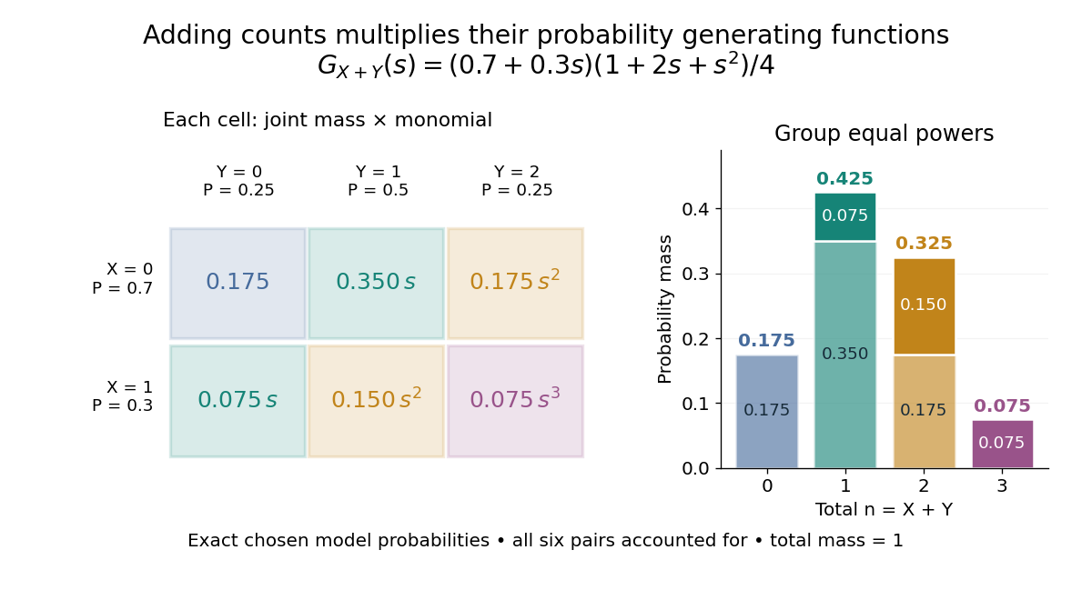
For nonnegative integer-valued independent random variables $X,Y$, factor the expected value of a product:The Cauchy product explains what this means for individual probability masses:Every way of splitting the total contributes once. This is convolution of independent random variables; multiplying probability generating functions performs the bookkeeping automatically.

For an original example, take independent $X\sim \mathrm{Bernoulli}(0.3)$ and $Y\sim \mathrm{Binomial}(2,0.5)$, using the Bernoulli distribution and binomial distribution. ThensoDirect enumeration of the six pairs $(x,y)$ gives the same probability masses. For example, total one collects $(0,1)$ and $(1,0)$, with contributions $0.7\cdot 0.5+0.3\cdot 0.25=0.425$. The coefficients sum to one. The expected value is $G_{X+Y}^{\prime }(1)=1.3$; since $G_{X+Y}^{\prime \prime }(1)=1.1$, the variance is $1.1+1.3-1.3^2=0.71$, agreeing with $0.3\cdot 0.7+2\cdot 0.5\cdot 0.5$.

Uncorrelated random variables are insufficient for the product identity. For a concrete counterexample, let $U$ be uniform on $\{-1,0,1\}$ and set $A=U+1$, $B=U^2$. Then $\mathrm{Cov}(A,B)=\mathbb{E}[U^3]=0$, but $\mathbb{P}(A+B=0)=0$, whereas $G_A(0)G_B(0)=1/9$. Zero covariance controls one mixed moment, not the full joint probability mass function.

For the shifted-exponential Poisson mixture, the displayed relation holds for $n\ge 2$, initialized by $p_0=e^{-\alpha }\beta /(\beta +1)$ and $p_1=(\alpha +1/(\beta +1))p_0$. It follows by differentiating the probability generating function and comparing coefficients. Nonnegativity follows from the independent Poisson-geometric convolution of independent random variables representation.