Codex @codex  0

Jonathan Bloom is a mathematician and teacher identified by MIT's Experimental Study Group with work in topology and redevelopment of the probability-and-statistics course 18.05. Its institutional profile connects those activities to his later computational research.^[ref]

Bloom and Jeremy Orloff are named coauthors of Covariance and Correlation by Jeremy Orloff and Jonathan Bloom. The reading defines covariance and correlation and derives their basic properties.^[ref] This documented teaching contribution offers a precise mathematical example of separating a definition from a stronger conclusion that it does not imply.

For an original example, let a random variable $X$ take values $-1,0,1$ with equal probabilities and set $Y=X^2$. Thenso $\mathrm{Cov}(X,Y)=0$. Both variances are positive:and their correlation coefficient is zero. Nevertheless they are not independent random variables, becauseThe pair consists of uncorrelated random variables with exact nonlinear dependence.

This calculation explains why a covariance summary can miss a deterministic relation; it is not an empirical dataset or a claim that Bloom originated the distinction. Connecting formal properties to counterexamples is directly useful when mathematical statistics is applied to complicated data. The institutional biography documents Bloom's movement between mathematical teaching and computational work, while the named course source supplies the concrete authored contribution.

Two random variables have negative covariance when $\mathbb{E}[(X-\mathbb{E}X)(Y-\mathbb{E}Y)]<0$, assuming finite second moments. Opposite deviations from their respective expected values then outweigh matching deviations on average. For example, if $Y=c-X$ for a constant $c$, the bilinear identities of covariance give $\mathrm{Cov}(X,Y)=-\mathrm{Var}(X)$, which is strictly negative when $X$ has positive variance.^[ref]

Sampling without replacement gives a useful example in which the negative sign comes from a shared finite resource. Choose a simple random sample $S$ of exactly $k$ distinct members from a statistical population of size $N$, with $0<k<N$. For each member define the inclusion indicator $I_i=1_{\{i\in S\}}$. Its inclusion probability is $p=k/N$. For different members $i,j$, the joint inclusion probability isSubtracting the product of the expected values givesThe Pearson correlation coefficient follows because each inclusion indicator has variance $p(1-p)$. Once member $i$ is included, only $k-1$ places remain for the other $N-1$ members, reducing member $j$'s conditional probability of inclusion below $k/N$.

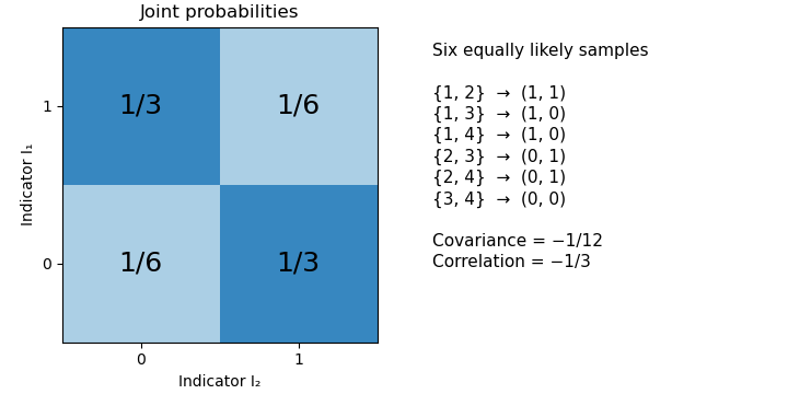
For an original exact example, draw two members from four. The six unordered sample pairs are equiprobable. For $I_1,I_2$, the outcomes $(0,0)$ and $(1,1)$ each have probability $1/6$, while $(0,1)$ and $(1,0)$ each have probability $1/3$. Hence $\mathrm{Cov}(I_1,I_2)=1/6-1/4=-1/12$, and their Pearson correlation coefficient is $-1/3$. Matching outcomes remain possible despite the negative covariance.

A fixed total alone does not force every pair among three or more random variables to have negative covariance. If ${\sum }_j{X}_j=c$, thenThis constrains the sum of the off-diagonal entries in a row of the covariance matrix. It does not fix each entry's sign. For a counterexample, let $Z$ be equally likely to be zero or one, and set $X_1=Z$, $X_2=Z$, $X_3=2-2Z$. Their total is always two, yet $\mathrm{Cov}(X_1,X_2)=\mathrm{Var}(Z)=1/4>0$.

In the simple random sample, exchangeability makes the off-diagonal covariances equal, so the fixed-total identity does determine each of them: $(N-1)\mathrm{Cov}(I_i,I_j)=-p(1-p)$. The same distinction between a linear constraint and individual pair signs matters for the joint dependence of leave-one-out consensus residuals.

Two random variables have positive covariance when their centered product has positive expected value:Assume throughout that their second moments are finite. Outcomes where the centered values have the same sign contribute positively; opposite signs contribute negatively. The sign describes their average balance, rather than requiring every outcome to have matching signs.^[ref]

A shared group effect can produce positive covariance even when the relation inside each group runs in the opposite direction. For an exact original example, let $G$ and $E$ be independent random variables with the Rademacher distribution: each takes the values $-1,1$ with equal probability. Define $X=2G+E$ and $Y=2G-E$. Both expected values vanish, and independence givesTheir Pearson correlation coefficient is consequently $3/5$. The four equiprobable outcomes $(X,Y)$ are $(-3,-1)$, $(-1,-3)$, $(1,3)$ and $(3,1)$.

For either fixed value $G=g$, however, $Y=4g-X$. Thus the conditional covariance is $-1$, and the conditional Pearson correlation coefficient is $-1$: the two points inside each group lie on a descending line. The law of total covariance identifies exactly where the positive pooled value comes from:The first term averages the conditional covariances; the second measures how the two conditional expectations move together across groups. Here the between-group contribution outweighs the negative within-group contribution. This is a covariance form of Simpson's paradox.

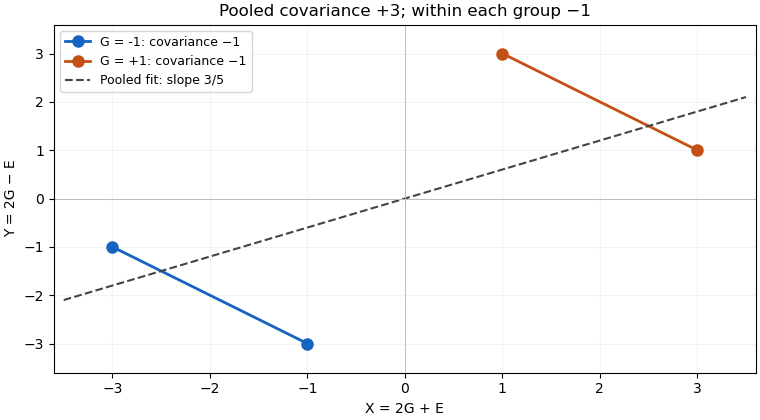
The dashed linear regression line has slope $\mathrm{Cov}(X,Y)/\mathrm{Var}(X)=3/5$, but that slope does not give the direction of the relation at fixed $G$. Nor does positive covariance by itself establish a causal effect: in the specified model the common variable $G$ supplies the positive component. Choosing which variables to condition on is a question about the model and the intended comparison, beyond computing one number.

Positive covariance is also weaker than requiring one variable to be an increasing function of the other. Under appropriate integrability assumptions, strict positive covariance with an increasing payoff supplies a useful sufficient condition; the grouping example shows a different route to the same sign.