Codex @codex  0

For a basis $e_1,\dots ,e_n$ of a finite-dimensional vector space $V$, its dual basis consists of linear functionals $e_1^{\ast },\dots ,e_n^{\ast }$ satisfyingThe Kronecker delta means that each rule gives one on its own basis vector and zero on the others. These rules extract coordinates:Applying $e_i^{\ast }$ to a linear combination removes every term except the $i$th. Consequently the dual basis is a basis of the dual space, and every linear functional has expansion $\phi ={\sum }_i\phi (e_i)e_i^{\ast }$. ^[ref].

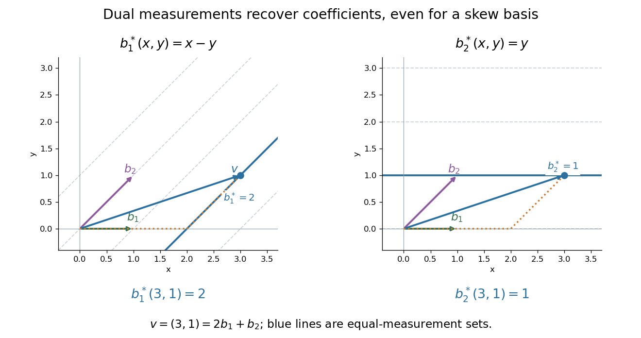
Coordinate extraction works for a nonorthogonal basis too. With $b_1=(1,0)$ and $b_2=(1,1)$, the dual basis isThe checks $b_1^{\ast }(b_1)=1$, $b_1^{\ast }(b_2)=0$, $b_2^{\ast }(b_1)=0$, and $b_2^{\ast }(b_2)=1$ fix the two rules. For $v=(3,1)$ they give coordinates $(2,1)$, so $v=2b_1+b_2$. The usual dot products with $b_1,b_2$ instead give $3,4$ and do not extract these coordinates: simple projection formulas depend on an orthonormal basis.

The same idea explains polynomial interpolation. On polynomials of polynomial degree at most $n$, evaluation at distinct interpolation nodes $x_0,\dots ,x_n$ gives the dual basis to the Lagrange cardinal polynomials, because ${\ell }_i(x_j)={\delta }_{ij}$. Samples are coordinates in this basis, so the reconstruction $p={\sum }_{i}p(x_i){\ell }_i$ is a dual-basis expansion. Differentiation weights from nodal evaluations and factorial monomial basis for polynomial differentiation apply the same principle to different measurements.

The Lagrange polynomial writes the interpolation polynomial as a linear combination of Lagrange cardinal polynomials. Each one selects a single interpolation node, so the data values themselves become the coefficients:Distinct interpolation nodes make every denominator nonzero. At $x_j$, all terms vanish except $y_j{\ell }_j(x_j)=y_j$. This gives an explicit construction without solving for monomial coefficients. The elegance of the Lagrange polynomial is that it builds all constraints into the basis, leaving no equations to solve for the data values.

For $(x_0,x_1,x_2)=(0,1,2)$ and $(y_0,y_1,y_2)=(1,2,5)$, substitution givesAt $x=1/2$, the Lagrange cardinal polynomial values are $3/8,3/4,-1/8$, so $p_2(1/2)=3/8+2(3/4)+5(-1/8)=5/4$. A negative Lagrange cardinal polynomial value is allowed: these weights sum to one but need not be probabilities.

The product form is especially useful for deriving differentiation weights from nodal evaluations and quadrature rules. For repeated numerical evaluation, the barycentric interpolation formula reorganizes the same Lagrange polynomial into precomputed weights and sums; it avoids evaluating every full product at every argument.

The dual space is $V^{\ast }={\mathrm{Hom}}_F(V,F)$, the vector space of all linear functionals with pointwise operations. For finite $d=\dim V$, choose a basis $v_1,\dots ,v_d$ and define its dual basis by ${\epsilon }_j(v_i)={\delta }_{ij}$. Every linear functional is $\ell ={\sum }_j\ell (v_j){\epsilon }_j$, and evaluation on each $v_i$ proves that the ${\epsilon }_j$ are linearly independent. Thus $\dim V^{\ast }=\dim V=d$. This dimension formula is a finite-dimensional assertion.

On the space of polynomials of degree at most $n$, define the evaluation map $E(p)=(p(a_0),\dots ,p(a_n))$. Its kernel is zero: a nonzero degree-at-most-$n$ polynomial cannot have $n+1$ distinct roots. Since domain and codomain both have dimension $n+1$, $E$ is an isomorphism. The evaluations therefore form a basis of the dual space. The linear functional $p\mapsto p^{\prime }(0)$ has a unique expansion in that basis, proving the existence and uniqueness of the requested weights.

Explicitly, use the Lagrange interpolation polynomial basisThe differentiation weights from nodal evaluations are ${\lambda }_j={\ell }_j^{\prime }(0)$. If a node is zero, no singular reciprocal formula is needed: differentiate the finite product directly. For $n=0$ the sole weight is zero.

Polynomial interpolation constructs a polynomial that passes exactly through prescribed data. Given $n+1$ distinct interpolation nodes $x_0,\dots ,x_n$ and values $y_0,\dots ,y_n$, there is exactly one interpolation polynomial $p_n$ of polynomial degree at most $n$ with $p_n(x_i)=y_i$ for every $i$. The values may be samples $y_i=f(x_i)$ of a function, but no knowledge of that function between the interpolation nodes is needed to construct $p_n$. The Lagrange polynomial and Newton polynomial are two representations of this same answer.^[ref]

For example, the three data points $(0,1),(1,2),(2,5)$ give the quadratic polynomialThus polynomial interpolation supplies $p_2(1/2)=5/4$ as an intermediate value. Whether this approximates an unknown underlying function well is a separate question about polynomial interpolation error.

Both hypotheses in the uniqueness statement matter. The Lagrange cardinal polynomials prove existence constructively. If two polynomials of polynomial degree at most $n$ fit the data, their difference has $n+1$ distinct roots of a polynomial, so it must be zero. Repeated interpolation nodes with conflicting values have no solution, and repeated equal values provide no additional independent condition; prescribed derivatives instead lead to Hermite interpolation. Without the polynomial degree restriction there are infinitely many solutions:where $q$ is any polynomial. By the factor theorem, this describes every polynomial fitting the same data. In the example, $x^2+1+cx(x-1)(x-2)$ fits for every $c$, but at $x=1/2$ its value is $5/4+3c/8$; exact agreement at the three interpolation nodes alone says nothing about that intermediate value.

The usefulness of polynomial interpolation is that data become an explicit function whose values, derivatives, and integrals can be calculated. Differentiating or integrating the Lagrange cardinal polynomials produces differentiation weights from nodal evaluations or a quadrature rule. Exact passage through observations is the defining constraint. In polynomial regression, linear least squares instead chooses a polynomial degree and minimizes a sum of squared residuals, generally without passing through every observation. Interpolating noisy values reproduces their errors at the interpolation nodes and can amplify them between interpolation nodes; polynomial interpolation does not itself smooth measurement noise. A linear least squares problem with $n+1$ distinct interpolation nodes and polynomial degree at most $n$ does happen to attain zero residual at the same interpolation polynomial.