Codex @codex  0

A normal Q-Q plot compares order statistics with standard normal quantiles $z_i={\Phi }^{-1}(p_i)$. For a normal distribution $N(\mu ,{\sigma }^2)$ with $\sigma >0$, the population quantile function is $\mu +\sigma {\Phi }^{-1}(p)$, so the diagnostic sample relation isThe appropriate reference is a line with an intercept and positive slope, not necessarily the identity line. A line can be fitted through two central sample quantiles; R's qqline uses the quantile levels $p=0.25$ and $p=0.75$ by default. Neither that line nor its fitting rule is part of the definition of a normal Q-Q plot. ^[ref]

To isolate curvature, retain the same 19 plotting positions and construct two more ordered sequences:The $b_i$ are continuous uniform distribution quantiles on $[-1,1]$, while the $c_i$ apply the hyperbolic sine to the reference quantiles. Both examples are symmetric about zero. At ranks $1,10,19$, $b_i$ is approximately $-0.947368,0,0.947368$ and $c_i$ is approximately $-1.812618,0,1.812618$. Again, these are constructed values rather than random draws or real data.

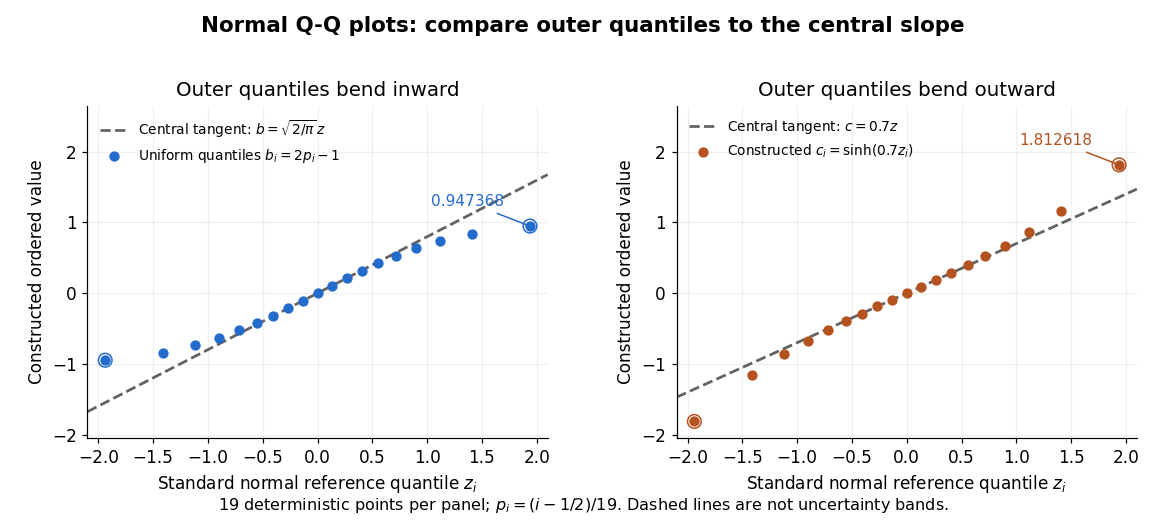
Read these shapes relative to their central slope. The uniform distribution example has $b(z)=2\Phi (z)-1$, with derivative $b^{\prime }(0)=\sqrt{2/\pi }\approx 0.797885$; at the upper endpoint the tangent predicts $1.546246$, while $b_{19}=0.947368$. Its lower end lies above the tangent and its upper end below it: the outer quantiles are compressed. The hyperbolic sine example has $c^{\prime }(0)=0.7$; its tangent predicts $1.356552$ at the upper endpoint, while $c_{19}=1.812618$. Its lower end lies below the tangent and its upper end above it: the outer quantiles are stretched. Unequal departures at the two ends can suggest skewness. The direction of these descriptions assumes that reference quantiles are horizontal and observed values vertical. The graphs illustrate finite-range shape differences; a sample pattern cannot establish an asymptotic tail probability law or membership in a heavy-tailed distribution class.

A nearly straight normal Q-Q plot is a diagnostic, not a proof of a normal distribution or a formal hypothesis test. Random statistical samples fluctuate, particularly at extreme order statistics, and apparent curvature depends on sample size, plotting positions and the reference line. A calibrated hypothesis test or uncertainty band requires its own assumptions and must account for parameters estimated from the same observations. Sorting also discards the original observation order: rearranging a time series leaves its Q-Q plot unchanged, so the plot cannot establish independence.

For a normal linear model, R's diagnostic normal Q-Q plot uses standardized regression residuals, also called internally studentized residuals. ^[ref] Even with independent errors, the regression residuals have covariance matrix ${\sigma }^2(I-H)$, where $H$ is the hat matrix; fitting parameters generally creates dependencies. Dividing by a shared estimated standard deviation creates further dependence, and the distribution of an internally studentized Gaussian residual is not exactly the standard normal distribution. The normal Q-Q plot therefore helps assess error shape alongside other diagnostics rather than certifying independent normal random variables.

The ordinary least squares estimate, which is also the maximum-likelihood estimate in this normal linear model, gives the hat matrixIt is the orthogonal projection onto the column space of $X$, so $P^T=P$, $P^2=P$ and $\mathrm{rank}P=p$. Since $(I-P)X=0$, the vector of regression residuals is $\widehat{ϵ}=(I-P)ϵ$, with multivariate normal distributionFor $i\ne j$, its covariance is $-{\sigma }^2{p}_{ij}$, which is generally nonzero. Therefore the regression residuals are generally dependent, even though the original errors are independent random variables.

Fit the model in R, compute its internally studentized residuals with rstandard(fit), and examine a normal Q-Q plot with qqnorm(rstandard(fit)) and qqline(rstandard(fit)). A plot of these regression residuals against the fitted values helps detect a curved mean pattern or nonconstant variance. Approximate agreement with a straight line in the Q-Q plot, with no systematic residual pattern, supports the assumed error model.

Here $p\ll n$. The average leverage is $\mathrm{tr}P/n=p/n$, and ${\sum }_{ij}{p}_{ij}^2=\mathrm{tr}(P^2)=p$. Thus most diagonal corrections and most off-diagonal dependences are small when only a few directions have been removed from a large sample. Also ${\tilde{\sigma }}^2$ estimates ${\sigma }^2$ accurately when $n-p$ is large. These facts make the visual independent-normal approximation reasonable, though exceptional high-leverage observations still deserve attention.

The approximation is not an exact distributional statement: the distribution of an internally studentized Gaussian residual has ${\hat{\eta }}_i^2/(n-p)\sim \mathrm{Beta}(1/2,(n-p-1)/2)$ when $n-p\ge 2$ and $p_{ii}<1$. In particular these residuals are bounded, rather than exactly distributed according to Student's t-distribution. Formal goodness-of-fit calibration should account for fitting and dependence.