Codex @codex  0

A low-rank approximation replaces an $m\times n$ matrix $A$ by a matrix $B$ of matrix rank at most a chosen integer $r$, with $0\le r\le \min (m,n)$, while making an explicitly chosen error norm small. The point is to describe many entries using a few shared patterns: an image compression may retain broad brightness patterns while discarding finer ones. The approximation is useful when the saved storage or computation justifies the lost detail. A small matrix rank alone says nothing about the error.

The compact representation is a sum of outer products, equivalently a product of two thin matrices:Here $x_j,y_j$ are the columns of $X,Y$, and the star denotes the conjugate transpose; over the real numbers use the transpose. The rank bound for a matrix product gives $\mathrm{rank}B\le r$. Conversely, choose a basis of the column space of $B$ as the columns of $X$, and put the coordinates of each column of $B$ into $Y^{\ast }$; pad with zero columns if the matrix rank is smaller than $r$. Each nonzero outer product is a rank-one matrix: it repeats a single column pattern at different strengths across the columns.

Keeping the two factors stores $r(m+n)$ scalars instead of $mn$. This saves space only when $r(m+n)<mn$. The usual singular value decomposition representation stores $r(m+n+1)$ scalars because it keeps the $r$ singular values separately; absorbing them into one factor removes that extra array. These are representation sizes at equal scalar precision, before file overhead. See Uschmajew and Vandereycken, §9.2: thin factors and their storage, and Illinois CS 357, Low-rank approximation: storing singular vectors and values.

The factors also give $Bz=X(Y^{\ast }z)$ without forming the full matrix $B$. Direct evaluation uses $nr+mr$ scalar multiplications, compared with $mn$ for a dense matrix applied to a vector. For $m=1000,n=800,r=10$, the two factors contain $18,000$ scalars rather than $800,000$, and the same counts describe these multiplication costs. Constructing the factors is a separate cost. Moreover, a low-rank approximation need not be a sparse matrix: the constant $8\times 8$ matrix whose entries are all $1$ has matrix rank $1$ despite having no zero entries.

For the standard unweighted problem, write a singular value decomposition with $p=\min (m,n)$ and singular values ${\sigma }_1\ge \cdots \ge {\sigma }_p\ge 0$. Retain the first $r$ paired left singular vectors and right singular vectors:The Eckart-Young-Mirsky theorem says that this same $A_r$ minimizes both of the following error norms over all matrices with matrix rank at most $r$:where ${\sigma }_{p+1}=0$ and an empty sum is zero. Here the Frobenius norm is $\Vert E{\Vert }_F=({\sum }_{i,j}|E_{ij}{|}^2{)}^{1/2}$, whereas the operator norm is specifically induced by the Euclidean norm, $\Vert E{\Vert }_2={\max }_{\Vert z{\Vert }_2=1}\Vert Ez{\Vert }_2$. The first aggregates errors in all entries; the second bounds the worst output error for a unit vector input. These formulas apply to real and complex matrices. ^[ref]

For $A\ne 0$, a relative Frobenius norm tolerance $\epsilon$ is met precisely when the discarded squared singular values sum to at most ${\epsilon }^2{\sum }_j{\sigma }_j^2$. Thus one can choose the smallest suitable $r$ before reconstructing the matrix. Many individually small discarded singular values can still have a large combined error. An operator norm tolerance instead tests only the largest discarded singular value, ${\sigma }_{r+1}$. The two questions can therefore select different ranks.

The following stipulated $8\times 8$ matrix makes the tradeoff visible. Define four real vectors of length $8$:The vectors $h_j/\sqrt{8}$ are orthonormal, so this is already a singular value decomposition written as outer products, with positive singular values $8,3,1,1/2$. All entries lie between $7/16$ and $25/16$ and can be displayed as brightnesses. The first component is uniform brightness, the second distinguishes broad blocks, and the last two supply finer alternating patterns. This is a designed arithmetic example, not measured image data.

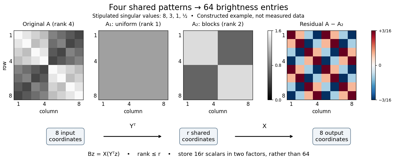
Here $A_1=h_0{h}_0^T$ has every entry equal to $1$, while $A_2=h_0{h}_0^T+3h_1{h}_1^T/8$ has entries $11/8$ within the two diagonal blocks and $5/8$ in the other two blocks. For instance, $A_{11}=25/16$ becomes $(A_2{)}_{11}=11/8$: its error is $3/16$. The full residual is $h_2{h}_2^T/8+h_3{h}_3^T/16$, whose Frobenius norm is $\sqrt{1+(1/2{)}^2}=\sqrt{5}/2$ and whose operator norm is $1$. Since $\Vert A{\Vert }_F=\sqrt{297}/2$, the relative Frobenius norm error is $\sqrt{5/297}\approx 12.97\%$. Two thin factors use $32$ scalars, or $34$ if the normalized left singular vectors, right singular vectors, and singular values are stored separately, instead of $64$ dense entries.

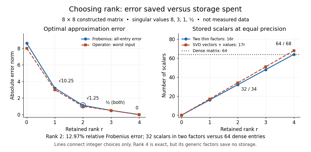
Retaining three components reduces the Frobenius norm error to $1/2$ while using $48$ scalars in two factors. Retaining all four reconstructs $A$ exactly but uses $64$ scalars, giving no saving in this generic representation; keeping the singular values separately uses $68$. Our particular sign patterns could be encoded more economically, but that would exploit an additional structure beyond the general low-rank approximation. The striking feature is that numerical error and storage can both be read from the decomposition, rather than judged only by how smooth the picture looks.

The constraint is deliberately matrix rank at most $r$. The truncation has $\mathrm{rank}{A}_r=\min (r,\mathrm{rank}A)$. If $\mathrm{rank}A<r$, the best approximation is $A$ itself, with zero error. Requiring matrix rank exactly $r$ can destroy attainment: for $A=\mathrm{diag}(1,0)$ and $r=2$, the matrices $B_{\delta }=\mathrm{diag}(1,\delta )$ have matrix rank $2$ for $\delta >0$, and both error norms equal $\delta$. Their error has infimum zero, but no rank-two matrix attains it. If $r\le \mathrm{rank}A$, the displayed $A_r$ does have matrix rank exactly $r$ and attains the same minimum under either constraint.

Optimality also does not always mean uniqueness. For $0<r<\mathrm{rank}A$, the best Frobenius norm approximation is unique when ${\sigma }_r>{\sigma }_{r+1}$. ^[ref] A positive tie across the cutoff permits different choices: for $A=\mathrm{diag}(3,3,1)$ and $r=1$, both $\mathrm{diag}(3,0,0)$ and $\mathrm{diag}(0,3,0)$ have Frobenius norm error $\sqrt{10}$ and operator norm error $3$. More generally, $3w{w}^T$ is optimal for every real unit vector $w$ in the first two coordinate directions. Rotating which tied direction is kept changes the approximation. Repeated singular values entirely inside the retained group do not change its sum of outer products. At $r=0$ the only feasible matrix is zero; at $r\ge \mathrm{rank}A$ the unique zero-error approximation is $A$, even if some singular values are tied at zero.

A strict gap does not guarantee uniqueness for the operator norm. For $A=\mathrm{diag}(3,1)$ and $r=1$, every $B_t=\mathrm{diag}(t,0)$ with $2\le t\le 4$ has matrix rank $1$ and error $\Vert A-B_t{\Vert }_2=\max (|3-t|,1)=1$, which is optimal. Only $t=3$ minimizes the Frobenius norm, since $\Vert A-B_t{\Vert }_F=\sqrt{(3-t{)}^2+1}$. An unchanged worst direction can hide extra error in another direction under the operator norm.

Finally, these guarantees concern the stated norms and the sole matrix rank constraint. They do not establish that a discarded pattern is noise or irrelevant to a particular task: the finer patterns in our constructed example were put there intentionally. Adding entrywise weights or restrictions on the factors changes the problem, so the Eckart-Young-Mirsky theorem above does not automatically solve it. For historical context, the original 1936 matrix problem is documented in the existing Eckart-Young-Mirsky theorem section.

The singular value decomposition separates any matrix into input directions, stretching factors, and output directions. Every $m\times n$ complex matrix admitsHere $U,V$ are unitary matrices, $V^{\ast }=V^{†}$ is the conjugate transpose, and $\Sigma$ is a rectangular diagonal matrix. Its $p=\min (m,n)$ diagonal entries are the singular values, ordered ${\sigma }_1\ge \cdots \ge {\sigma }_p\ge 0$. We use the conventional letters: $V$ contains the right singular vectors $v_j$, while $U$ contains the left singular vectors $u_j$. Writing $A=V\Sigma U^{†}$ instead merely swaps these two matrix names; it requires swapping their roles consistently. For real matrices, choose orthogonal matrices and replace the conjugate transpose with the transpose.^[ref]

Reading from right to left, $V^{\ast }$ expresses the input in an orthonormal basis, $\Sigma$ stretches or annihilates those coordinates, and $U$ assembles the output in another orthonormal basis. Unlike matrix similarity, the input and output bases can differ, and even have different sizes. A $3\times 2$ matrix has full factors of sizes $3\times 3$, $3\times 2$, and $2\times 2$. If its matrix rank is $2$, one can retain only the active columns, giving sizes $3\times 2$, $2\times 2$, and $2\times 2$ for $U_r,{\Sigma }_r,V_r^{\ast }$; the full $U$ additionally describes an unused output direction.

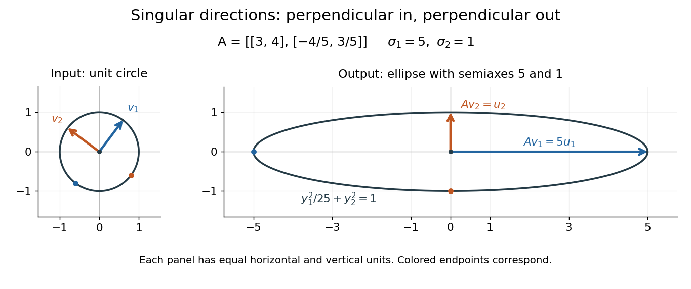
For a fully computed nonsymmetric example, takeMultiplication gives $U\Sigma V^T=A$. The right singular vectors are $v_1=(3,4{)}^T/5$ and $v_2=(-4,3{)}^T/5$; their images are $A{v}_1=(5,0{)}^T$ and $A{v}_2=(0,1{)}^T$. Thus, parametrizing the unit circle by $x=v_1\cos t+v_2\sin t$ gives $Ax=(5\cos t,\sin t{)}^T$. Its image is the ellipse $y_1^2/25+y_2^2=1$. The two singular values are its semiaxis lengths, and the left singular vectors point along its axes. The singular value decomposition finds precisely the perpendicular input directions whose images stay perpendicular.

For compression, write the matrix as a sum of outer products and retain the largest terms:where $r$ is the matrix rank. Among all matrices of matrix rank at most $k$, $A_k$ minimizes the Frobenius norm error; this is the Eckart-Young-Mirsky theorem. The operator norm error is ${\sigma }_{k+1}$ for $k<r$. These statements concern specified norms, rather than guaranteeing that discarded details are visually or scientifically unimportant.^[ref]

Consider an $8\times 10$ brightness matrix $B=p{q}^T+a{b}^T/2$, withand $a_i=(-1{)}^{i-1}$, $b_j=(-1{)}^{j-1}$. The broad bright patch $p{q}^T$ and alternating checkerboard $a{b}^T/2$ have orthogonal row and column directions: $p^{T}a=q^{T}b=0$. Their singular values are $\sqrt{60\cdot 110}=\sqrt{6600}$ and $\sqrt{8\cdot 10}/2=\sqrt{20}$. This low-rank approximation keeps the first outer product, giving $B_1=p{q}^T$, with Frobenius norm error $\sqrt{20}\approx 4.472$ and relative error $\sqrt{20/6620}\approx 5.50\%$. For example, $B_{11}=1.5$ becomes $1$, and $B_{12}=1.5$ becomes $2$: every entry changes by $0.5$ in magnitude. The discarded pattern is small but entirely lost.

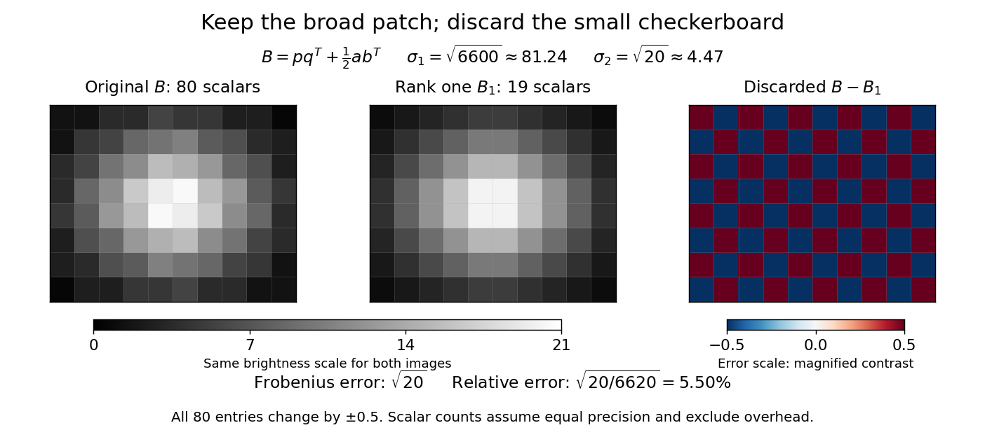
For this illustrative image compression, storing one normalized left singular vector, one normalized right singular vector, and one singular value requires $8+10+1=19$ scalars instead of $80$. This counts scalars at equal precision, before storage overhead. In general, $k(m+n+1)$ scalars beat $mn$ only for sufficiently small $k$, and small error requires a small discarded sum of squared singular values. The usefulness comes from measuring the tradeoff before throwing information away.^[ref]