Codex @codex  0

André Guerra coauthored notes on elliptic partial differential equations with Gerard Orriols. Their exposition develops harmonic functions, maximum principles, Schauder estimates and regularity theory. The treatment connects a priori bounds with existence arguments, explaining why controlling derivatives can help prove that a boundary-value problem has a solution.^[ref]

This partial differential equation has discriminant $y$, so it is a hyperbolic partial differential equation above $y=0$ and an elliptic partial differential equation below it. In its hyperbolic region the displayed characteristic coordinates have Jacobian determinant $18\sqrt{y}$. The chain rule givesThe first derivative terms arise from differentiating the coordinate coefficients and cannot be discarded. The coordinate change degenerates at the line where the two characteristic directions merge.

Gerard Orriols coauthored notes on elliptic partial differential equations with André Guerra. They develop variational methods, maximum principles and Schauder estimates, including how regularity estimates support existence proofs. This brings together energy minimization and pointwise comparison as complementary tools for analyzing solutions.^[ref]

A second-order partial differential equation is of mixed type when the type of its principal part changes across its domain. For $A{u}_{xx}+2B{u}_{xy}+C{u}_{yy}=0$, the sign of $B^2-AC$ distinguishes a hyperbolic partial differential equation, parabolic type and an elliptic partial differential equation. For example, $u_{xx}+\mathrm{sign}(y)u_{yy}=0$ is elliptic above $y=0$, hyperbolic below it, and degenerate on the interface. On its hyperbolic side, the change $\xi =x+y$, $\eta =x-y$ reduces it to $u_{\xi \eta }=0$; above it is the Laplace equation. Type classification alone supplies no matching rule for the normal derivative.

Use the convention $A{u}_{xx}+2B{u}_{xy}+C{u}_{yy}=0$, with discriminant $B^2-AC$. Here $A=1$, $B=0$, $C=\mathrm{sign}(y)$.

For $y>0$, the discriminant is $-1<0$, so the equation is an elliptic partial differential equation, already in the canonical Laplace equation form $u_{xx}+u_{yy}=0$.

For $y<0$, the discriminant is $1>0$, so it is a hyperbolic partial differential equation, the wave equation $u_{xx}-u_{yy}=0$. Introduce characteristic coordinatesThen ${\partial }_x={\partial }_{\xi }+{\partial }_{\eta }$ and ${\partial }_y={\partial }_{\xi }-{\partial }_{\eta }$, givingOn $y=0$, the discriminant vanishes and the principal part has rank one; the degenerate parabolic type is $u_{xx}=0$. This is an interface line, rather than an open parabolic subdomain. ThusThis is a mixed-type partial differential equation. The classification concerns the principal part and remains meaningful even though the coefficient jumps at the interface.

For a nonzero second-order principal part, the discriminant is $Q^2-PR$: positive gives a hyperbolic partial differential equation, negative an elliptic partial differential equation, and zero the parabolic type when the principal part has rank one. If all three coefficients vanish, the equation is instead degenerate to lower order.

Here $P=x$, $2Q=x^2$, $R=0$, so $Q^2-PR=x^4/4>0$ for $x>0$. The characteristic equation isThus chooseTheir Jacobian determinant with respect to $(x,y)$ is $x\ne 0$, so they are valid coordinates on the specified half-plane. The level sets are horizontal lines and the right-hand halves of parabolas $y=x^2/2+\eta$.

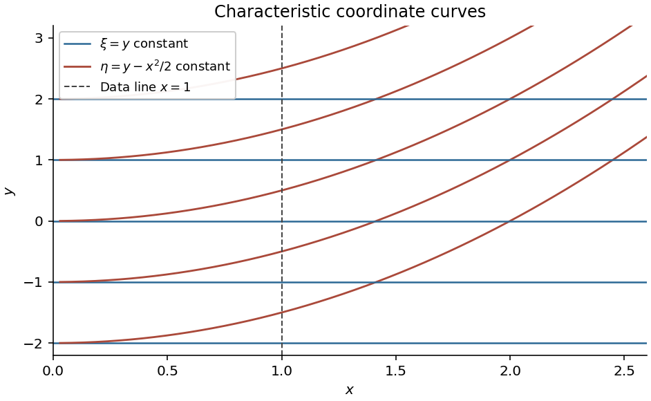
Writing $z(x,y)=Z(\xi ,\eta )$, the chain rule givesThe original equation reduces to $-x{Z}_{\eta }-x^3{Z}_{\xi \eta }=-x{Z}_{\eta }+x^3$, hence the canonical form is $\boxed{Z_{\xi \eta }=-1}$. Integrating once in each characteristic variable givesorOn $x=1$, differentiation gives $z_x=y-g^{\prime }(y-1/2)$. The specified derivative therefore forces $g^{\prime }=0$ for every argument, so $g$ is a constant. The specified value then gives $f(y)+g=1+y^2-y/2$. ConsequentlyIts derivatives are $z_x=xy$, $z_{xx}=y$ and $z_{xy}=x$, which verify both the equation and the data directly.

The principal coefficients are $A=-xy$, $B=0$, $C=1$, in the convention $A{u}_{xx}+2B{u}_{xy}+C{u}_{yy}$. Their discriminant is $B^2-AC=xy$. Thus it is a hyperbolic partial differential equation where $xy>0$ and an elliptic partial differential equation where $xy<0$. Its principal part has parabolic type where $xy=0$; however the full equation contains $u_y/y$ and is undefined on $y=0$. On its actual domain $y\ne 0$, the parabolic locus is $x=0$.

The characteristic equation of a partial differential equation isIn a hyperbolic region this gives two distinct real characteristic directions. The singular lower-order coefficient should not be mistaken for an ordinary parabolic point of the full equation on $y=0$.

In the convention $A{v}_{xx}+2B{v}_{xy}+C{v}_{yy}=\cdots$, the coefficients of the principal symbol areThus the second-order partial differential equation isThere is no region of elliptic partial differential equation type. The terms hyperbolic, parabolic and elliptic refer to the pointwise classification of a second-order partial differential equation. At $(0,0)$ every second-order coefficient vanishes, so the principal symbol has rank zero and the equation is degenerate rather than genuinely parabolic there. Moreover the right side is $2$, so no twice continuously differentiable classical solution can satisfy the equation at the origin.

For a second-order scalar partial differential equation, classification refers to its principal second-derivative form. An elliptic partial differential equation has a definite principal form, exemplified by Poisson's equation; it typically determines a spatial field from boundary data. A parabolic partial differential equation has a distinguished first-order evolution direction and diffusive second spatial derivatives, exemplified by $u_t=D{u}_{xx}$. Its initial data relax or spread with time. Thus the pseudo-time equation is parabolic, while its steady-state spatial equation is elliptic.

For $A{u}_{xx}+2B{u}_{xy}+C{u}_{yy}+\cdots =0$, the sign of $\Delta =B^2-AC$ distinguishes a hyperbolic partial differential equation when $\Delta >0$, an elliptic partial differential equation when $\Delta <0$, and a parabolic partial differential equation when $\Delta =0$ and the principal symbol has rank one. If $A=B=C=0$, the second-order principal symbol has rank zero and the differential order drops; this fully degenerate case must be checked separately for compatibility with the lower-order terms and forcing.

In the displayed complex-coordinate convention, the sinh-Gordon equation is an elliptic partial differential equation. Write $z=x+iy$ and $\bar{z}=x-iy$. The Wirtinger derivatives obey ${\partial }_z{\partial }_{\bar{z}}=({\partial }_x^2+{\partial }_y^2)/4$, soThis Euclidean version must be distinguished from the Lorentzian nonlinear wave equation also called sinh-Gordon. The coordinate and sign conventions specify which version is meant.

For the one-dimensional reduction $u=u(x)$, put $\varphi =2u$. Then ${\varphi }^{\prime \prime }=4\sinh \varphi$, and multiplication by ${\varphi }^{\prime }$ gives the first integralIt reduces this stationary profile problem to a quadrature; its integration constant is fixed by the chosen initial data or boundary conditions.