Codex @codex  0

Arbitrage pricing theory relates expected returns to systematic factor loadings and their risk premiums. With idiosyncratic noise, a diversification or asymptotic argument needs additional assumptions. With no idiosyncratic noise and spanned factors, the formula is an exact consequence of law of one price: portfolios matching factor exposures can differ only by a constant payoff, which absence of arbitrage forces to be zero.

An orthogonal rotation of factors leaves $L{L}^T$ unchanged and hence preserves the model covariance. It proves rotational nonidentifiability of the unrestrained factor loadings. Choose an orientation for interpretability, for example varimax rotation, or impose identifying restrictions in a confirmatory model. An oblique transformation permits correlated factors: if $L$ becomes $LH$, their covariance becomes $H^{-1}{H}^{-T}$, preserving the same shared covariance.

A latent factor is an unobserved coordinate introduced to explain shared variation among measurements. In an orthogonal factor model, latent factors have variance one and are mutually uncorrelated, with coefficients specified by the factor loadings. They differ from a regression factor, which is a categorical predictor. A fitted covariance alone generally leaves the latent factor orientation undetermined; factor rotation gives equivalent representations.

Treat the forty-person convenience sample as a pilot, then develop and validate the measure in its intended population. Start by defining whose organizational ability the questionnaire measures and who answers it: lecturer self-reports and student ratings are different measurements. Specify the relevant activities and context. Discuss the candidate items with lecturers and appropriate users, seek expert review, and use cognitive interviewing to find ambiguous wording, double-barreled items and irrelevant content. This establishes content validity rather than assuming that correlations alone identify the intended construct.

Recruit a larger, better-targeted sample covering relevant roles, disciplines and institutions. A convenience sample of adults who cannot meaningfully judge lecturers' organization is not made suitable simply by increasing its size. Plan the sample size using plausible factor loadings, communalities, number of dimensions and indicators, response distributions, missingness and required estimation stability, preferably with simulation. Forty observations for sixteen items offer limited grounds for a stable generalizable structure; no universal participants-per-item cutoff makes this analysis automatically impossible or automatically adequate. If students rate the same lecturers, recognize that the ratings are clustered rather than independent lecturer-level observations.

Check missing responses, item distributions, scoring direction and correlations, identifying redundant or poorly functioning items. If the underlying dimensions are not already well specified, use exploratory factor analysis to model shared variation among items. Principal component analysis instead forms combinations explaining total observed variation; it is not the same latent measurement model. Choose a suitable common-factor estimator, such as principal axis factoring, or maximum likelihood estimation when its assumptions are credible. For ordered response categories, consider an ordinal estimator and polychoric correlations, while checking whether category counts support their estimation. Do not treat those correlations as assumption-free.^[ref]

Choose the number of factors using parallel analysis, the scree plot, substantive interpretation and the quality of the resulting model, rather than an eigenvalue-one rule alone. Parallel analysis compares the observed eigenvalues with a reference generated from uncorrelated data of comparable dimensions; its implementation must match the chosen correlation and extraction approach.^[ref] Use oblique factor rotation if organizational dimensions can plausibly correlate. Inspect factor loadings, cross-loadings, communalities, factor correlations and model discrepancies, and retain enough substantively relevant indicators for each dimension. Do not repeatedly delete items solely to improve numerical fit at the expense of coverage.

After developing the structure, test it using confirmatory factor analysis in an independently recruited validation sample, with the proposed structure fixed beforehand. Splitting the existing forty participants would not solve the shortage of information. Evaluate model fit and uncertainty, measurement reliability, test-retest reliability where stability is intended, and evidence for construct validity using related, distinct and relevant behavioral measures. Check measurement invariance before comparing scores across groups. Report alternative plausible models, all item decisions, sampling limitations and the distinction between an initial exploratory instrument and an independently validated measure.

Use factor analysis when several observed measurements may reflect fewer unobserved dimensions, such as related questionnaire items about planning, prioritization and record keeping. A common-factor model separates shared variation represented by latent factors from item-specific variation. Factor loadings describe how measurements relate to those latent factors; communalities summarize their shared-variance contributions.

Exploratory factor analysis investigates a structure not yet fixed; confirmatory factor analysis evaluates prespecified measurement restrictions, preferably in independent data. Extraction, factor count and factor rotation affect interpretation, so report them and justify the sample and measurement assumptions. A statistically convenient factor solution does not alone establish construct validity or demonstrate the existence of a literal psychological mechanism. The distinction from principal component analysis is the common-versus-total-variation objective, and from cluster analysis the modeling of measurement relationships rather than the grouping of cases.

Let $B$ be the $n\times m$ matrix of factor loadings, so $r=a+Bf$. A zero-cost portfolio $v$ with $1^{T}v=0$ and $B^{T}v=0$ again has constant financial payoff $v^{T}a$. Absence of arbitrage impliesTaking expectations givesIf $[1B]$ has full column rank, a unit-cost portfolio with zero exposure to all factors exists and earns the certain rate ${\lambda }_0$. For each $j$, choose a zero-cost portfolio with loading one on factor $j$ and zero on the others; its expected return is ${\lambda }_j$. Hence these coefficients are the rewards per unit systematic exposure, or factor risk premiums, with the financial payoff measured per unit of the chosen factor normalization. A traded risk-free asset fixes ${\lambda }_0$ to its return. Changing the scale or basis of the factors changes the coordinates of the risk premiums but leaves asset prices unchanged. With deficient rank, only the spanned factor directions are identified and the coefficients need not be unique.

Factor analysis models a large set of correlated measurements using a smaller collection of shared latent factors and variable-specific variation. A classical orthogonal factor model isTake $q<p$, centered errors, and positive specific variances for the inverse-covariance and likelihood formulas below. The factor loadings form the $p\times q$ matrix $L$, and the model covariance isThus for $i\ne k$, $\mathrm{Cov}(X_i,X_k)={\sum }_j{L}_{ij}{L}_{kj}$; the common latent factors explain off-diagonal correlation. The communality of variable $i$ is $h_i^2={\sum }_j{L}_{ij}^2$, and $\mathrm{Var}(X_i)=h_i^2+{\psi }_i$. For standardized variables this is $1=h_i^2+{\psi }_i$. The specific variance represents measurement noise or genuinely unshared variation; it is not another common latent factor.

This differs from principal component analysis. A principal component maximizes projected total variance and is a determined linear score after choosing its direction; a factor model attempts to explain shared covariance while reserving diagonal specific variance. Low-dimensional PCA truncation can help initialize a factor fit, but it does not justify setting all specific variances to zero. Latent factors are unobserved, not directly observed scores. When the latent factors and the errors are jointly Gaussian, their conditional mean iswhich supplies one factor-score estimate, with remaining uncertainty. This follows from the block conditional normal formula in Question 1; it does not make the latent factor uniquely recoverable from one observation.

For the Gaussian likelihood, use the empirical covariance $S_0=n^{-1}{\sum }_i(x_i-\bar{x})(x_i-\bar{x}{)}^T$. Fit the factor model by minimizing $\log |L{L}^T+\Psi |+\mathrm{tr}(S_0(L{L}^T+\Psi {)}^{-1})$ subject to admissible specific variances. Other approaches estimate communalities and extract latent factors from the reduced correlation matrix. Choose $q$ using substantive plausibility, a scree plot, fitted residual correlations and model-fit assessment. Under local identifiability, a likelihood goodness-of-fit count for the covariance model iswhere the subtracted rotational dimension must be removed from the loading parameter count. This count alone does not establish identifiability, and boundary fits with zero specific variance need special care.

Factor rotation addresses interpretability and nonuniqueness. For every orthogonal matrix $Q$, replace $(L,F)$ by $(LQ,Q^{T}F)$; then $(LQ)(LQ{)}^T=L{L}^T$, so the fit is unchanged. The absolute orientation of unrestrained latent factors is therefore not identified by the covariance. Varimax rotation chooses orthogonal axes favoring a simple pattern of large and small squared loadings. Oblique rotation can permit correlated latent factors, provided their covariance is transformed consistently. Sign changes and permutations are further harmless relabelings; an interpretation must state its chosen convention.

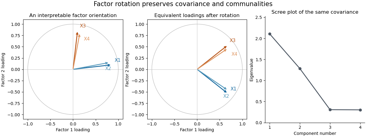
The sketch uses four standardized hypothetical measurements sharing two orthogonal latent factors. Rotating the factor coordinates changes the loading descriptions while preserving every implied covariance and communality; the scree plot belongs to that same constructed covariance matrix. Factor analysis separates shared variation from specific variance, and its latent factors require an identifying or interpretive orientation.

A common-factor extraction method based on iteratively estimating shared variance and the associated factor loadings. It differs from principal component analysis, whose components summarize total observed variation.