Maximum likelihood estimation is a method of statistical estimation: within a specified statistical model, choose the statistical parameter values that maximize the likelihood function of the observed data. For a parameter set and observations , its exact requirement isThe equality requires an attained, finite maximum; a supremum approached only at an excluded boundary is not enough. The resulting rule is a maximum-likelihood estimator. The likelihood function uses a probability mass function for discrete data and a probability density function for continuous data. See MIT 18.05, Reading 10b, sections 3 and 3.2.
The direction of the comparison is the interesting part: hold the observations fixed and vary the statistical parameter. Ten independent Bernoulli trials with eight successes and two failures give the maximum-likelihood estimate , as derived in log-likelihood. This chooses the member of the statistical model that assigns the greatest mass to that outcome. It does not assert an posterior probability that this parameter value is true. Bayesian statistics combines the same likelihood function with a prior distribution to obtain a posterior distribution; maximum a posteriori estimation maximizes that posterior mass or density instead.
The method turns many fitting tasks into one maximization problem. In the normal distribution model with known variance, it recovers the sample mean and ordinary least squares, while binomial regression and Poisson regression use different sampling assumptions to build their own likelihood functions. The log-likelihood turns independent contributions into a sum, exposing score equations and observed information. A peak's location gives an estimate; its shape records how much the observed data distinguish nearby parameter values.
Existence, uniqueness, bias, and statistical consistency are separate questions. Normal mean and variance maximum-likelihood estimators include a variance estimate with bias, likelihood supremum at an excluded boundary gives nonexistence, and the Neyman-Scott incidental parameter problem gives inconsistency. The usual asymptotic normality of a maximum likelihood estimator requires assumptions: a consistent estimator at an interior true parameter in a fixed finite-dimensional model with identifiability, sufficient smoothness and control of log-likelihood derivatives, and finite nonsingular Fisher information. A common parameter-independent support of a probability distribution is part of a standard sufficient framework; see Rigollet, MIT 18.650, Maximum Likelihood Estimation, slides 22-23. This is a description of the regular setting, not a complete theorem's hypotheses. The exact endpoint limit for a shifted exponential distribution shows why changing support can produce a different rate and a nonnormal limit. These properties do not follow just from maximizing a function.
In his 1922 paper in the Royal Society's Philosophical Transactions A, R. A. Fisher explicitly distinguished likelihood from probability and described choosing the parameter values with greatest likelihood. Section 6 also discusses comparing likelihoods after giving the maximum value one, the convention used in the figures here. See Fisher, On the Mathematical Foundations of Theoretical Statistics, section 6, pp. 326-328, DOI 10.1098/rsta.1922.0009.
For independent normal distribution observations with mean and variance , put , . The Fisher-Neyman factorization theorem makes a sufficient statistic, since the likelihood is proportional to . Its logarithmic derivative has numerator . When , this changes sign once on the positive half-line and gives the displayed global maximum-likelihood estimator. The zero sample is a probability-zero exception with unbounded likelihood as .
For independent -variate multivariate normal observations with unknown mean and unrestricted positive-definite covariance matrix, the centered scatter has rank at most . If it is singular, choose the mean to be the sample mean and shrink the covariance on a null direction of the scatter. The quadratic likelihood term stays fixed while the determinant tends to zero, so the density likelihood tends to infinity. Thus a nonsingular covariance maximum likelihood estimate exists only when the centered scatter is positive definite; for a nonsingular Gaussian population this occurs almost surely exactly when .
On a compact parameter space, suppose the expected log-likelihood is continuous, uniquely maximized at the true parameter, and the normalized empirical log-likelihood converges uniformly in probability to its expectation. On the compact complement of every neighbourhood of the truth, the expected criterion has a strictly positive gap below its maximum. Uniform approximation by less than one-third of this gap excludes every empirical maximizer from that complement. Identifiability and nonnegativity of Kullback-Leibler divergence supply the unique expected maximizer. The proof works for any measurable choice of maximizer.
A shifted exponential distribution has location estimate equal to the sample minimum and rate estimate given above, for a nondegenerate sample of at least two observations. The minimum exceeds the true location on average by . The residual sum above the minimum is gamma with shape , so the rate estimate has expectation for and infinite expectation at . The estimated location plus reciprocal rate is the unbiased sample mean.
For independent observations with having exponential distribution of known rate , the likelihood increases in until the smallest observation, so the maximum-likelihood estimator is . Its survival function is for . Therefore has exactly the unit-rate exponential distribution for every sample size. This gives statistical consistency and a one-sided nonnormal limit with rate , illustrating how a support endpoint changes usual regular likelihood asymptotics.
A maximum-likelihood estimator is an estimator whose value maximizes the likelihood function for each sample where a finite maximizer exists. Before observation, is a random variable (the choice of maximizer must be a measurable function); after observation, is the numerical maximum-likelihood estimate. A formula must specify the allowed parameter set, including whether its endpoints belong to it.
For ten independent Bernoulli trials, write . On the closed parameter interval , the binomial proportion maximum-likelihood estimator is . Eight successes give the estimate . If , the likelihood is and has its unique maximum at ; if , it is and has its unique maximum at . On the open interval these two samples have no maximum-likelihood estimate: the supremum is one, but it is not attained. This is the same issue as likelihood supremum at an excluded boundary.
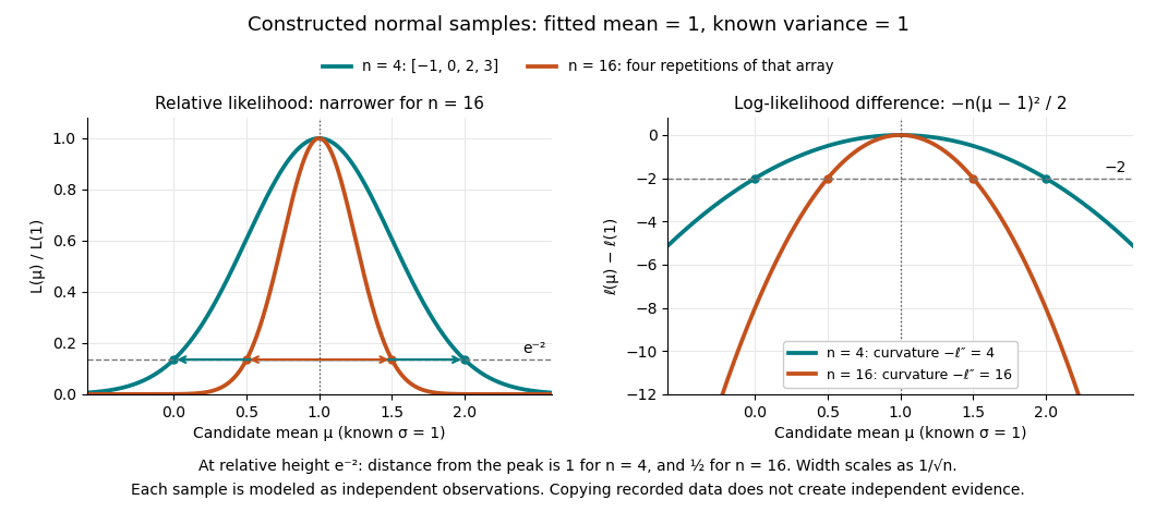
A complete continuous example uses independent and identically distributed random variables with unknown mean and known standard deviation one. Their likelihood function and log-likelihood areThe sum of squared deviations separates asbecause . The first term is fixed in , so the unique maximum-likelihood estimator is the sample mean . This also proves the equivalence with ordinary least squares for this model. With the constructed observations , the sample mean is one and the residual sum of squares is ten; henceAt or , the log-likelihood is two below its peak, so the likelihood ratio to the fitted value is . The absolute likelihood at the peak is , a joint density value, not the probability of observing exactly those four real numbers.
The following figure compares that sample with a constructed sixteen-observation sample consisting of four repetitions of the displayed four values, modeled as sixteen independent draws. Both fits have sample mean one, butThus the observed information is four times as large for as for . The distance from the peak at relative height decreases from one to : the width scales as . This is a comparison of two stipulated samples; merely copying recorded observations would not create new independent evidence.
Even uniqueness needs checking. If the Bernoulli distribution success parameter is written with , eight successes give two maximum-likelihood estimates, , because both give the same probability distribution. The problem is a failure of identifiability. The special cases below show other ways an MLE can have bias or fail the usual asymptotic normality.
A likelihood need not attain its supremum when the parameter space excludes a boundary point. For example, with parameter and a zero Poisson count, the likelihood is strictly decreasing and has no maximum. Extending the parameter space to include zero gives an extended maximum-likelihood estimate there. A proposed estimator formula involving that boundary value must distinguish the extended estimate from an actual maximizer in the original space.
For independent observations, the likelihood decreases as on , so its maximizer is the sample maximum almost surely. Its exact distribution is for . This proves consistency and an endpoint error of order , with the displayed exponential limit. Parameter-dependent support violates the usual regularity condition behind nondegenerate square-root-sample-size normal limits; the ordinary interior score is not centered.
A growing number of nuisance parameters can prevent a maximum-likelihood estimator of a common parameter from being consistent. With two independent normal observations of mean per group, the profiled variance estimate tends to half the true variance, because each unknown mean is estimated using only two observations.
For density on , , the interior likelihood function increases without bound as approaches the sample minimum. The extended-likelihood estimator is that minimum. An arbitrary finite reassignment of the density at the endpoint can eliminate an attained finite maximum, so the endpoint convention must be stated.
For independent observations from the exponential distribution with rate , the log-likelihood is , soThe central limit theorem and delta method give
A maximum-likelihood fitted value is a response mean or probability evaluated at a maximum-likelihood estimate. In a parametric mean model it is .
For independent and identically distributed random variables , the maximum-likelihood estimators areThe first is unbiased, while .
If maximizes a likelihood and the target parameter is , a maximum-likelihood estimate of is , with the usual interpretation when is not one-to-one.
For a fixed observed sample , a likelihood function iswhere is the probability mass function or probability density function of the observations under the statistical parameter . All densities must be defined relative to the same parameter-independent dominating measure. The sample is fixed; the parameter is the function's argument. With independent and identically distributed random variables, the joint mass or density factors as . This definition and the distinction between sampling probability and parameter uncertainty are explained in MIT 18.05, Reading 10b, sections 3 and 3.2.
For an observed ordered sequence of ten independent Bernoulli trials containing eight successes and two failures, each success contributes and each failure contributes , givingIf the observation is instead only the total count , its binomial distribution probability mass function sums over the possible ordered sequences:The raw heights differ: at they are approximately and . Their maximum-likelihood estimates are identical. More generally, multiplication by any finite positive constant independent of leaves the maximizing parameter values and all likelihood ratios unchanged. Multiplication by a parameter-dependent factor can change the MLE; dropping such a factor is not justified. Relative likelihood height sets the peak to one, without making the area under the curve one.
Normalization of is over possible data values for each fixed parameter. It imposes no requirement that . For example, the ordered Bernoulli trials likelihood above hasIts integral is not one, and its values are not posterior probabilities for . When the Bayesian posterior is defined, Bayes' theorem multiplies the likelihood by a prior density and normalizes that product. Choosing to normalize a likelihood function alone is an additional choice, such as using a uniform prior in those parameter coordinates, rather than part of the definition of likelihood.
For observations with a probability density function, the probability of an exact sample point is zero. If a scalar density is continuous at the observed value , thenThus the density compares probabilities of small, equal observation intervals at different parameter values; it is not itself the probability of that exact real number. The equal-width factor is independent of the parameter. This gives visual intuition for density likelihoods, as in MIT 18.05, Reading 10b, section 4. The normal distribution example in maximum-likelihood estimator makes the comparison explicit. If only rounded intervals are recorded, their integrated probabilities give the exact observation likelihood; using midpoint densities is an approximation.
The log-likelihood is the natural logarithm of the likelihood function:For positive finite likelihood, the natural logarithm is a strictly increasing function, so the maximizing parameter values are unchanged. Set where ; the same ordering then includes zero-likelihood boundaries whenever a positive finite maximum exists. For independent and identically distributed random variables, a product becomes a sum,This makes derivatives simpler and avoids forming products of tiny numbers in floating-point arithmetic. These equal-maximizer and additive formulas underlie the worked calculations in MIT 18.05, Reading 10b, section 3.1.
For the ordered sample of eight successes and two failures in likelihood function, on ,The score equation gives , hence . The negative second derivative proves strict concavity, so this is the unique interior maximum. Both counts are positive, so , while inside: the same point is the unique global maximum on . Counting only successes adds to the log-likelihood, leaving both derivatives and the MLE unchanged. For all-success or all-failure samples, the boundary analysis in maximum-likelihood estimator applies instead of an interior score equation.
The two panels below compare successes out of ten Bernoulli trials. Their peaks are at . The left panel uses relative height; the right panel uses the log-likelihood difference from each peak. These are the same comparison on two scales:A difference of means relative height , and a difference of means ; the log-likelihood scale makes small relative heights easier to see. Neither vertical axis is a parameter probability density function. The zero likelihood endpoints have log-likelihood and are outside the finite vertical range in the right panel.
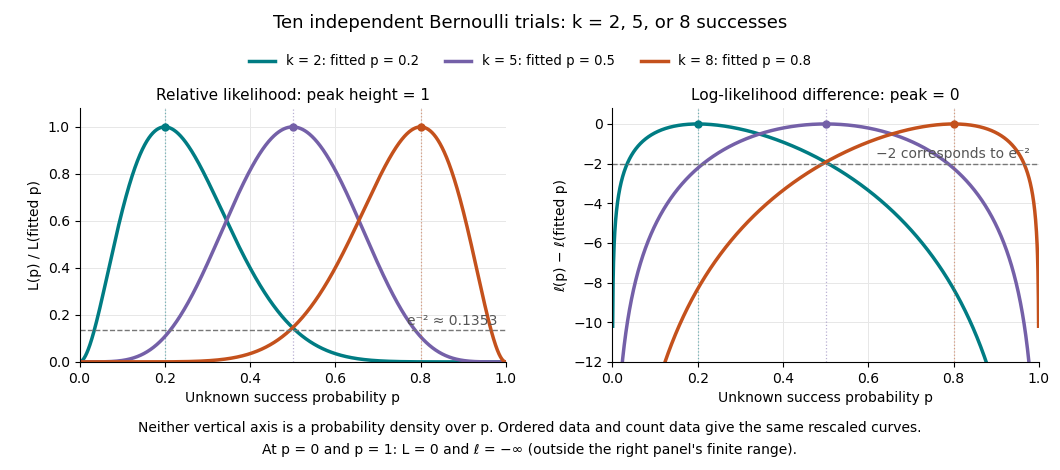
Ten Bernoulli trials: relative likelihood heights and log-likelihood differences share the same peaks
. Details. Multiplying a likelihood function by a positive parameter-independent constant adds a constant to its log-likelihood. Subtracting its peak removes that constant. This is why the ordered-data and count-data curves coincide in this figure after rescaling. When differentiable, the gradient of the log-likelihood is the score function; the negative Hessian matrix is the observed information. A solution of a score equation still needs checking against other stationary points and boundaries: maximizing the log-likelihood does not automatically make it concave.
If a statistic T has marginal density depending on a parameter of interest but not on a nuisance parameter, that density gives a likelihood for the interest parameter. It is obtained by integrating out other observed coordinates. In contrast, profile likelihood maximizes the full likelihood over the nuisance parameter. This sampling-statistic construction is different from Bayesian model evidence, which integrates parameters against a prior. No prior is required for a nuisance-free sampling marginal.
A conditional likelihood evaluates the conditional distribution of the observed data given a specified statistic. If that distribution does not involve a nuisance parameter, it permits inference about the remaining parameter without estimating the nuisance parameter. The conditioning statistic need not be ancillary; possible information loss must be assessed within the model. Conditional maximum likelihood maximizes this function.
For a regular two-parameter exponential family, condition on the sample mean of the nuisance canonical statistic. Exponential tilting to its observed value and the saddlepoint density approximation give a nuisance-statistic density proportional to times its large-deviation exponential. Dividing the joint likelihood by this density gives the profile log-likelihood plus the displayed adjustment, up to a data-only constant. The sign is positive. This construction assumes an interior saddle with positive curvature and a sufficiently regular nonlattice density; conditioning on a lattice statistic requires the corresponding mass approximation.
An observed-data likelihood integrates the full-data statistical probability density over unobserved values, rather than inserting arbitrary values or discarding incomplete records. When the observation pattern is random, its mechanism belongs to the joint observation model unless the conditions for an ignorable missingness mechanism permit its factor to be omitted.
A Bayesian deviance is minus twice the log-likelihood, with any chosen additive data-only constant held consistent across the models being compared. Its Bayesian posterior expectation measures average fit. In the deviance information criterion, evaluating it at a parameter's posterior mean also enters the effective complexity penalty. This likelihood-based convention differs by a data-only constant from a saturated-model exponential-family deviance when a common saturated model exists.
A conditional likelihood function conditions on an initial observation or another specified statistic. In an autoregressive model, conditioning on the first observed state avoids modeling its initial density. For Gaussian transitions, maximizing this likelihood is a regression problem; treating an autoregressive coefficient as known changes the exact distribution of an estimated mean.
For a parameter of interest and nuisance parameter , the profile likelihood isIt compares values of after fitting the nuisance parameter as favourably as possible at each value.
For parameter of interest , constrained nuisance fit , and suitable ancillary sample coordinates , this adjustment includes both nuisance observed information and a sample-space Jacobian determinant. The derivative holds fixed. Implicit differentiation of the constrained nuisance score function gives the equivalent expression . The semicolon distinguishes data-coordinate differentiation from parameter differentiation. Omitting the Jacobian requires an additional justified simplification; the information adjustment alone is not universal.
For independent Inverse Gaussian distributions with shape and mean , the constrained and full nuisance maximum-likelihood estimates both equal , giving a unit sample-coordinate Jacobian determinant. The nuisance observed information there is . Hence subtracting half its logarithm from the profile log-likelihood replaces the coefficient of by . For a nonconstant sample the modified fit is .
For independent exponential distributions with means and a nonconstant fixed design, put . The constrained maximum-likelihood estimate is and the profile log-likelihood is . Use the ancillary statistic to specify sample coordinates. At fixed , the Jacobian determinant , while . Therefore the modified profile likelihood satisfiesThe adjustment is independent of . Keeping only the observed information adjustment would miss this cancellation.
For independent and in shape-rate notation, has density proportional to . Its distribution is nuisance-free in lambda. The nuisance maximum is , so substituting into the full likelihood gives the same interest-parameter log-likelihood up to a parameter-free term. Equality here is special to the common-scale structure, not a general equality of profiling and marginalization.
The logarithm of the profile likelihood is the full log-likelihood evaluated at the nuisance fit constrained to the specified parameter of interest. It preserves likelihood ratios and maximizers, but is not generally a normalized sampling log-density. Conditioning and integrating out nuisance parameters are different operations.
Articles by others on the same topic



Maximum Likelihood Estimation (MLE) is a statistical method used to estimate the parameters of a statistical model. The core idea behind MLE is to find the parameter values that maximize the likelihood function, which quantifies how likely it is to observe the given data under different parameter values of the statistical model. ### Key Concepts: 1. **Likelihood Function**: Given a statistical model characterized by certain parameters, the likelihood function is defined as the probability of observing the data given those parameters.