A statistical model is identifiable when distinct parameter values determine distinct probability distributions. In a nonidentifiable parameterization, data can at most estimate combinations of parameters that remain unchanged along each equivalent parameter set.
Nonregular identification at a flat mean map occurs when different parameter values give different probability distributions, yet the first derivative of the observable mean vanishes at a parameter of interest. Identifiability is a property of the entire parameter-to-distribution map; a first-order sensitivity calculation can miss it.
Consider an original statistical model with independent observationsThe cubic mean map is a strictly increasing function, so equality of the normal distributions implies equality of . The model is globally identifiable, including at . Nevertheless, the single-observation score function and Fisher information areThus does not imply nonidentifiability. The rank is zero at the origin and one at every nonzero nearby point. This is precisely why a regular-point assumption matters: Rothenberg's local identification criterion assumes constant information-matrix rank in a neighborhood.[ref]
Maximum likelihood estimation gives , using the real cube root. At the true value zero, write with a standard normal random variable . ThenThis is an exact sampling distribution identity for every , not merely a convergence in distribution statement. The estimation error has scale and a nonnormal shape. At a fixed nonzero , the usual delta method instead gives asymptotic variance ; that approximation cannot be extended uniformly through zero.
An exact confidence interval through a cubic mean map follows by applying the strictly increasing function to both endpoints of the ordinary known-variance confidence interval for the mean:Here is the quantile function of the standard normal distribution. The transformed interval has exact coverage for every . When and the observed sample mean is zero, the 95% interval is approximately . Multiplying by 64 halves its width at that observed mean. A first-order interval based on dividing by the zero mean-map derivative would fail instead.
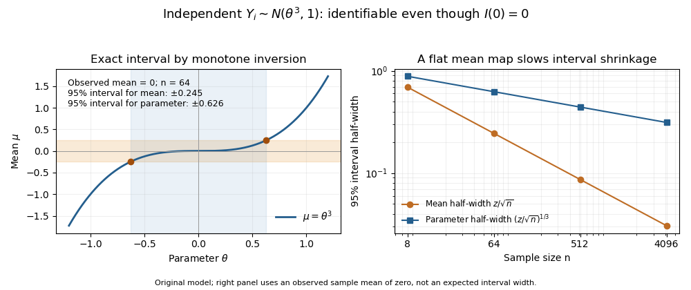
Cubic mean map and exact confidence-interval scaling at an observed sample mean of zero; original normal-observation model
. Details. 
Quantity-specific identifiability asks whether a chosen function of a model's parameters is determined by the observable probability distribution, even when the complete parameter vector is not. For model and target , the criterion isEquivalently, the target must be constant on each class of observationally equivalent parameters. This separates identification of a scientifically meaningful quantity from reconstruction of every internal parameter. Thomas J. Rothenberg's primary treatment explicitly distinguishes identification of individual parameter components from that of a full system.[ref]
Identification in Parametric Models by Thomas J. Rothenberg. §5, printed p.586, individual-parameter discussion and Theorem8
For an original example, let observations have a Poisson distribution with mean , where . Parameter pairs and give exactly the same observable law. The sum is identifiable, but is not: its values are and . With independent observations, the sample mean estimates the sum with variance . More observations can improve that estimate without distinguishing the two allocations.
Identifiability from linear observations gives a useful exact criterion. Suppose the observation law identifies and contains no additional information about . A linear target is identifiable exactly when belongs to the row space of . To prove this, observationally equivalent parameter differences lie in the kernel of a linear map . The target is unchanged for every such difference precisely when is orthogonal to that kernel, which is equivalent to membership in the row space. If , the target can be recovered as .
A deterministic geometric analogue appears in additional measurements and anatomical identifiability: measured perimeter can determine the surface area of the stipulated cuboid family even when exchanging its two horizontal side labels remains invisible. The target and the allowed model class must be stated.
Identification is not the same as good precision. A formally identifiable target can still be weakly constrained by finite noisy data. Conversely, a nonidentifiable target requires additional assumptions or observations, rather than merely more repeated data from the same indistinguishable law.
Identifiability from linear observations asks which features of an unknown vector are fixed by observing . Two parameter vectors are observationally equivalent exactly when their difference lies in the kernel of a linear map :Thus the full vector is identifiable precisely when , equivalently when has full column matrix rank. Repeating the same rows can improve precision in a noisy measurement without increasing this rank.
A linear target requires less information. It is identifiable if and only if is in the row space of . If , then , so the target is recovered directly. Conversely, an identifiable target must vanish on every observationally invisible difference: for every . Orthogonality to the kernel is exactly row-space membership. This is a concrete instance of quantity-specific identifiability; the primary identification literature also treats identification of individual parameter components by rank conditions.[ref]
Identification in Parametric Models by Thomas J. Rothenberg. §5, printed p.586, Theorem8
For an original example, supposeBoth and fit perfectly. Their difference is a multiple of , which spans the kernel. The target is identified, whereas takes values 8 and 9 and is not. A new independent measurement of restores full identification; another copy of does not.
The same distinction applies to a statistical model with known positive-definite covariance matrix : two parameters give the same observable law precisely when their means agree. A Moore-Penrose pseudoinverse selects one solution when the system is underdetermined, but that numerical convention does not show that the selected vector is the unique physical parameter. Additional restrictions must be justified as assumptions, not silently supplied by a solver.
In a normal linear model with an intercept and factor effects, set the effect of one factor level to zero. The intercept then denotes that reference level's mean, and the remaining effects are contrasts to it. The constraint removes redundant statistical parameters without altering the fitted mean space.
Articles by others on the same topic
There are currently no matching articles.