Define a signed offset so that the accelerating region adds kinetic energy . This convention concerns this gap; collector contact fields belong in the effective . An Electron emitted with initial kinetic energy and undergoing identical excitation losses reaches the grid withEach loss excites a fresh chemical atom initially in its ground state. These are repeated payments of the same excitation cost. The index counts events along an Electron trajectory, not the ordinal number of an atomic excited state. The outgoing energy also does not locate the last collision: after an early collision an Electron can regain enough kinetic energy to cross the barrier.
At fixed , let be the normalized initial-energy probability density function within the ensemble of Electrons reaching the grid, and the conditional probabilities for losses within that ensemble. Then the ideal collection law isTake and exclude paths with insufficient kinetic energy for a loss at its actual collision position. The weights contain collision positions and rates, mean free paths and angular acceptance. This equation is a bookkeeping model, not a derivation of those weights. Multiplying all incident particles by one constant transmission is an additional approximation; real transmission and can vary with .
One analytical extreme assumes , one-dimensional motion and an immediate loss whenever the kinetic energy reaches . With , and , the number of losses and remaining kinetic energy areHere is the floor function. Collection switches off for an interval of width after each reset, then recovers; the pattern repeats every . For , and , an applied gives , and rejection, whereas gives , and collection. With the dips disappear in this idealization. With no collisions, there is only a single collection onset. Both limits expose the separate roles of loss and filtering.
To draw a smooth illustrative curve, extend this periodic rule mathematically to all and convolve it with a chosen normal distribution of voltage jitter, of standard deviation :Here is the standard normal cumulative distribution function. Each summand is the smoothed indicator of the accepted interval . The result satisfies and has period . For the figure choose and plot only well beyond the startup region. This is a chosen phenomenological curve, not a Boltzmann equation transport prediction or a fit to measured electric current. Its symmetric troughs center on , rather than the reset voltages . Finite excitation rates, several loss channels, space charge, initial angular and energy spreads, and real electrode geometry can change the trough shape and phase; a single convolution does not solve these effects.
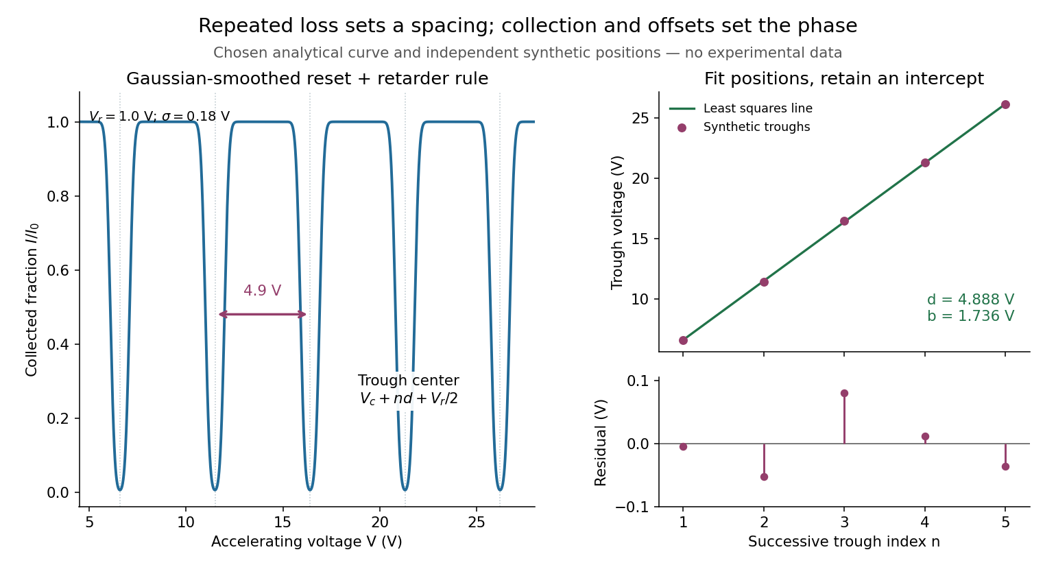
Illustrative repeated-loss collection and an independent synthetic spacing fit
. Left: the chosen Gaussian-smoothed threshold model, with , , and . Right: separately chosen synthetic trough positions, their ordinary least squares fit and residuals. The points are not extracted from the left curve or a historical trace. Source. Details.
Articles by others on the same topic
There are currently no matching articles.