A useful Franck-Hertz energy-loss model separates three operations: accelerating an Electron, losing a discrete energy in an inelastic collision, and selecting the surviving Electrons with a retarding collector. The collector measures an accepted fraction of an outgoing energy distribution. This makes the experiment a small inverse problem: the electric current depends on both the collision physics and the readout.
For a deliberately simple one-channel model, let be the incoming kinetic energy, and let be the probability that one encounter excites the chemical atom. Set for and otherwise. The conditional probability distribution of outgoing kinetic energy is the discrete loss kernelHere is the Dirac delta function. The kernel has unit integral, no negative outgoing energy, and mean outgoing kinetic energy . It neglects the small recoil loss in an elastic collision, other excitation channels and ionization. The threshold permits excitation; it does not require above threshold. In particular, choosing a single here isolates the characteristic channel discussed above without claiming it is mercury's lowest possible excitation.
For Electrons directed normally toward an ideal planar collector, a retarding electric potential difference imposes the barrier . Write its transfer as , where is the Heaviside step function and the positive elementary charge. Thus a perfectly sharp loss need not produce a sharp drop in electric current: the drop also depends on where the outgoing energy lies relative to the barrier. For an oblique incident Electron at angle to the normal, the same planar model instead tests ; angular scattering can change collection even at unchanged total kinetic energy.
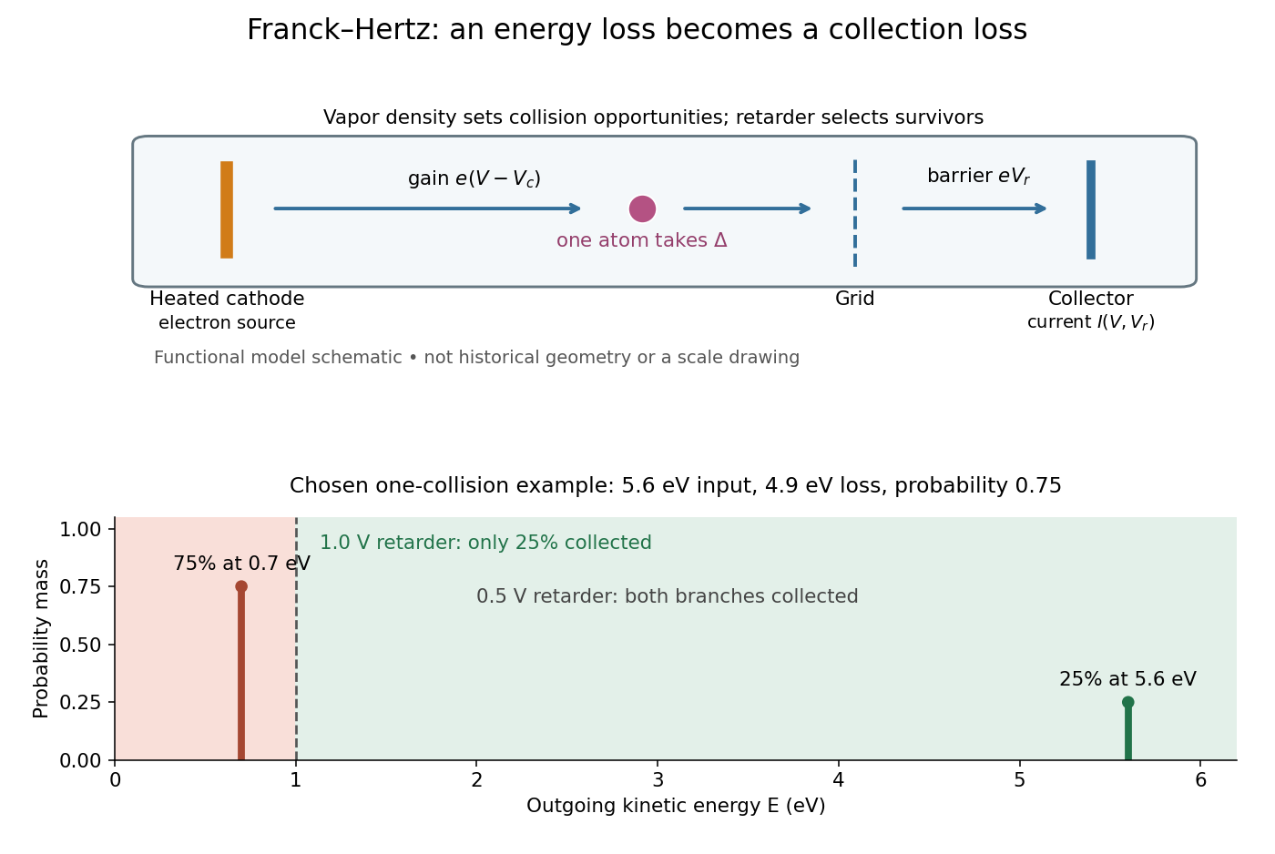
Franck-Hertz energy-loss model: separate acceleration, loss and collection
. Original functional schematic, not a scale reconstruction of a historical tube. The lower panel applies an ideal normally incident retarder to the explicitly chosen one-collision example. Equal vertical strokes mark outgoing energies; their labeled weights give probabilities. Source. Details.
For example, choose a monoenergetic incoming beam with , and . After one encounter, have and have . A retarder collects only , whereas a retarder collects ; here is the incident electric current with fixed geometrical acceptance and no background. The mean outgoing kinetic energy is , independently checked by . These are chosen inputs and calculated fractions, not historical measurements.
More generally, let be the normalized outgoing probability density function at a fixed accelerating electric potential difference , for the normally incident idealization. A retarding scan givesThe second equation follows by differentiating the lower integration limit, with Dirac delta functions understood for sharp beams. It explains why an integrated collector readout can reveal an energy distribution. With angles present it probes the distribution of normal kinetic energy; finite instrumental resolution smooths it, and numerical differentiation amplifies noise. Keep the incoming beam fixed during this scan. A scan of changes itself and cannot be differentiated by the same inversion formula.
Define a signed offset so that the accelerating region adds kinetic energy . This convention concerns this gap; collector contact fields belong in the effective . An Electron emitted with initial kinetic energy and undergoing identical excitation losses reaches the grid withEach loss excites a fresh chemical atom initially in its ground state. These are repeated payments of the same excitation cost. The index counts events along an Electron trajectory, not the ordinal number of an atomic excited state. The outgoing energy also does not locate the last collision: after an early collision an Electron can regain enough kinetic energy to cross the barrier.
At fixed , let be the normalized initial-energy probability density function within the ensemble of Electrons reaching the grid, and the conditional probabilities for losses within that ensemble. Then the ideal collection law isTake and exclude paths with insufficient kinetic energy for a loss at its actual collision position. The weights contain collision positions and rates, mean free paths and angular acceptance. This equation is a bookkeeping model, not a derivation of those weights. Multiplying all incident particles by one constant transmission is an additional approximation; real transmission and can vary with .
One analytical extreme assumes , one-dimensional motion and an immediate loss whenever the kinetic energy reaches . With , and , the number of losses and remaining kinetic energy areHere is the floor function. Collection switches off for an interval of width after each reset, then recovers; the pattern repeats every . For , and , an applied gives , and rejection, whereas gives , and collection. With the dips disappear in this idealization. With no collisions, there is only a single collection onset. Both limits expose the separate roles of loss and filtering.
To draw a smooth illustrative curve, extend this periodic rule mathematically to all and convolve it with a chosen normal distribution of voltage jitter, of standard deviation :Here is the standard normal cumulative distribution function. Each summand is the smoothed indicator of the accepted interval . The result satisfies and has period . For the figure choose and plot only well beyond the startup region. This is a chosen phenomenological curve, not a Boltzmann equation transport prediction or a fit to measured electric current. Its symmetric troughs center on , rather than the reset voltages . Finite excitation rates, several loss channels, space charge, initial angular and energy spreads, and real electrode geometry can change the trough shape and phase; a single convolution does not solve these effects.
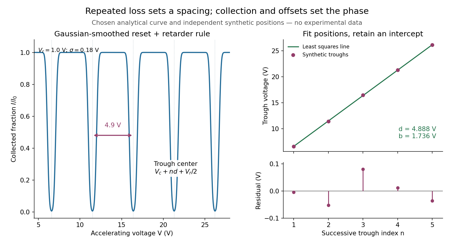
Illustrative repeated-loss collection and an independent synthetic spacing fit
. Left: the chosen Gaussian-smoothed threshold model, with , , and . Right: separately chosen synthetic trough positions, their ordinary least squares fit and residuals. The points are not extracted from the left curve or a historical trace. Source. Details.
Fit the positions of successive, consistently defined troughs by linear regression, . A constant intercept absorbs the contact potential difference, collection phase and initial energy effects; estimates the repeated loss expressed as a voltage. Subtracting successive positions cancels . A line fit uses every position and leaves residuals that can reveal curvature or a misidentified trough. It still assumes that the phase is constant over the fitted range and that all troughs belong to the same loss channel.
For an original numerical example, choose and synthetic positions . Their successive spacings are . The ordinary least squares formulas giveThe fitted residuals are , with zero sum and zero index-weighted sum. Their residual sum of squares is . If independent, equal-variance, zero-mean errors describe these positions, the residual variance estimate is and the slope standard error is . Thus the inferred model loss is with conditional standard error . These errors summarize only the chosen position scatter; a voltage-scale error or a drifting collection phase is not included. Adjacent spacings share a position error and are therefore correlated even when position errors are independent.
The offset has a sharper identifiability limitation. Even if a constant-phase model were exact, an initial beam kinetic energy shifts the troughs by . For the symmetric illustrative curve, . The transformation , leaves every trough position unchanged. Measuring alone therefore cannot determine the contact potential difference. Relabeling also changes by without changing . An independent offset calibration and a justified collection model are needed before turning a first trough into an excitation threshold. Varying tests this model's predicted half-voltage shift of the trough centers; it is a diagnostic prediction of this chosen curve, not a universal correction for experimental minima.
Articles by others on the same topic
There are currently no matching articles.