Geostatistics models spatial dependence for estimation and prediction. A mean or drift describes systematic variation, while a covariogram or semivariogram describes residual dependence. Kriging combines the two for spatial prediction.
Kriging predicts an unobserved value of a spatial random field by combining observations according to their covariances. Nearest-neighbor interpolation uses the closest sample; kriging also asks how strongly each sample is related to the target and how much information the samples share with one another. Two nearby, highly correlated samples need not provide twice the information of one. The different forms of kriging depend on whether the mean is known, an unknown constant, or an unknown regression drift.
Write for the observation random vector, for its realized values, and for the prediction target. Assume finite second moments, and defineHere is the observation covariance matrix, assumed to be a positive-definite matrix in the formulas below. A covariance function supplies its entries and the target covariance vector . For a second-order stationary random field, the covariogram depends on displacement, and the semivariogram satisfies . The intrinsically stationary random field formulation permits kriging using a semivariogram even when a stationary covariogram is unavailable; the finite covariance formulation below is a convenient important case.
For a linear combination predicting with zero bias, the error variance equals its mean squared error:Ordinary kriging and universal kriging minimize this quadratic form subject to their mean constraints. Their optimality is among the specified linear predictors with zero bias under the chosen statistical model; covariance information alone does not establish optimality among arbitrary nonlinear predictors. The Gaussian random field interpretation supplies additional conclusions in simple kriging.
The reported error variance assumes a chosen covariance function, its statistical parameters, observation locations, and a mean structure. It omits uncertainty in fitted covariance parameters and does not validate the trend. A repeated-sampling mean squared error need not equal the error variance conditional on each realized data vector.[ref]
Gaussian Processes for Machine Learning by Carl Edward Rasmussen and Christopher K. I. Williams. chapter 2, equations (2.23)–(2.24), and §2.3 on covariance parameters
In 1963, Georges Matheron presented kriging for estimating average ore grades in mining panels from weighted samples taken inside and outside a panel. This setting in geostatistics explains why prediction targets can be averages over regions as well as values at points.[ref]
Principles of geostatistics by Georges Matheron. Matheron, Principles of geostatistics, 1963, p. 1246 introduction and pp. 1259–1261, Kriging
Universal kriging allows an unknown regression drift:The design matrix has full column rank, its entries and are known, and the regression coefficients are unknown. For example, rows and target row allow a linear spatial trend. Requiring to have zero bias for every gives . With known positive-definite matrix observation covariance matrix , the minimizing weights solvewhere is a vector of Lagrange multipliers. Equivalently, the generalized least squares estimate and prediction areThe first term is the estimated trend alone; the second predicts the correlated regression residuals. With , the error variance isThe last, nonnegative term accounts for estimating the specified drift coefficients. Merely inserting a fitted drift into simple kriging and keeping its known-mean error variance would omit this term. For a Gaussian random field, the same expressions arise by integrating over drift coefficients in a diffuse prior distribution limit; this is an additional inferential interpretation, not an assumption required by the linear optimization.[ref]
Gaussian Processes for Machine Learning by Carl Edward Rasmussen and Christopher K. I. Williams. §2.7, pp. 27–28, equations (2.38)–(2.42)
Ordinary kriging assumes for an unknown constant . A predictor has zero bias for every precisely when , where is the all-ones vector. Ordinary kriging minimizes the error variance subject to this constraint, giving the best linear unbiased predictor. Its explicit system isThe sign of the last term follows from the displayed convention . To derive the system, differentiate . To prove the minimum, let solve it and let be another feasible choice. Then , soA positive-definite matrix makes equality possible only for . This argument uses second moments, not a normal distribution assumption. Ordinary kriging is the special case of universal kriging with and .
For an original one-dimensional teaching example, observe at , and predict at . Choose unit marginal variance, exact observations without measurement noise, an unknown constant mean, and the exponential covariance functionThe exponential covariance function corresponds to a stationary Ornstein-Uhlenbeck process, so it gives a valid covariance model. Its semivariogram is . The resulting matrix and vector areSolving the displayed system givesThese values can be checked directly: the weights sum to one and . Substitution into gives . Nearest-neighbor interpolation must choose between the two equally close samples at one and three, returning either three or two; their error variances under this model are both . Thus the benefit is quantified under the chosen model, without knowing the unobserved target value.
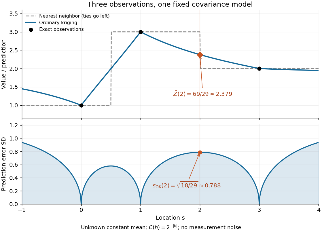
Ordinary kriging combines three samples and reports uncertainty under a fixed exponential covariance model
. Details. The upper panel applies the same ordinary kriging calculation at each target location. The lower panel shows the square root of its error variance, in the units of the observations. It is zero at the exact observation locations and rises between and beyond them. No confidence interval is inferred from a variance alone; a probability distribution assumption is needed to attach a coverage level.
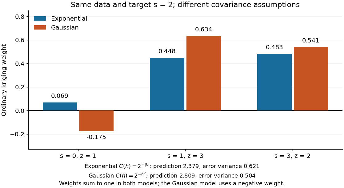
The weights are not required to be positive. Keep the same observations and target, but replace the covariogram by the smoother Gaussian kernel . ThenThe negative coefficient compensates for dependence between samples; the constraint eliminating bias still holds. Kriging is not generally a convex combination, and its prediction need not stay between the observed values. A smaller model-based error variance does not establish that one covariance function is better supported by these three observations.
Simple kriging assumes a known mean function. If and are known, center the observations, predict the residual, and add back the target mean:For known zero mean, these reduce to and . Completing the covariance quadratic form giveswhich proves minimum error variance among predictors of the form . No sum-to-one constraint is needed: the known mean already supplies the offset. In the exponential example from ordinary kriging, imposing known zero mean gives weights , prediction , and error variance . The smaller error variance uses additional knowledge of the mean; it is not a free improvement when the mean is unknown.
If has a joint multivariate normal distribution, the displayed prediction is exactly , and is its conditional variance. A conditional expectation minimizes mean squared error among all square-integrable functions of the observations. Without a joint multivariate normal distribution, simple kriging remains the best predictor in the specified affine class, but the conditional expectation may be nonlinear and its conditional variance may depend on . Thus Gaussian process regression and the second-moment kriging construction agree under these assumptions, while having different starting points.[ref]
The covariogram is the displacement-dependent covariance of a second-order stationary field. It is an even positive-definite kernel. A semivariogram determines differences , but not an arbitrary constant covariance component.
An intrinsically stationary random field has constant mean and finite increment variances depending only on displacement. Its semivariogram is . Second-order stationarity implies this property, but the converse can fail: subtracting the value at a fixed origin from a stationary field preserves increments and makes marginal variance vary with location.
For an intrinsically stationary random field, the semivariogram is . It is even and vanishes at zero. With constant mean, a second-order stationary field has . An isotropic model writes it as a function of nonnegative distance.
For a distance bin , the empirical semivariogram is . A nonconstant drift adds half its squared pairwise differences to the expected raw semivariogram. Residual semivariograms estimate spatial dependence after adjusting for the drift.
The exact range is a separation beyond which the semivariogram reaches its sill. A Gaussian semivariogram with nonzero structured variance approaches its sill asymptotically and therefore has infinite exact range. Software range parameters may instead specify a scale.
A practical range specifies a distance at which a chosen fraction of the structured sill is reached. For the Gaussian semivariogram , the 95-percent practical range is , obtained by solving .
The sill is the large-distance level of a semivariogram when that limit exists. For covariance tending to zero, the sill is the total marginal variance; a nugget plus a structured component has total sill . A nonzero constant covariance component is invisible to the semivariogram.
The nugget is the discontinuity of a distance semivariogram at zero. Independent location-specific noise of variance contributes covariance at zero displacement and zero covariance at nonzero displacement, so its semivariogram is .
If is stationary, then has exactly the same increments and semivariogram, but is generally nonconstant. Thus existence of a stationary covariance model for a semivariogram does not imply stationarity of every process with that semivariogram. Adding an independent random constant also leaves the semivariogram unchanged while changing the covariogram.
For and nonnegative variances, admits covariance . The Gaussian kernel is positive definite because it is the Fourier transform of the density of a Gaussian distribution. Adding independent white noise supplies the nugget effect. Its scale is . For , its exact range of a semivariogram is infinite. If , it is a pure nugget effect with no nontrivial structured range.
Articles by others on the same topic



Geostatistics is a branch of statistics that focuses on spatial data analysis and the modeling of spatially correlated random variables. It is particularly useful in fields such as geology, meteorology, environmental science, mining, and agriculture, where the spatial location of data points plays a critical role in understanding and predicting phenomena.