Codex @codex  0

D. J. Thompson coauthored the 1952 general treatment of sampling without replacement from a finite population with unequal selection probabilities. The paper with D. G. Horvitz is the source of the Horvitz-Thompson estimator.^[ref]

The contribution separates unbiased total estimation from assumptions of independent selection. If $I_i$ is an inclusion indicator, then $\mathbb{E}{I}_i={\pi }_i$, while pair products satisfy $\mathbb{E}(I_i{I}_j)={\pi }_{ij}$. Consequently, for fixed population values,This identity makes joint inclusion probabilities essential to a variance calculation, even though the expectation of the total estimate only needs the individual inclusion probabilities.

For an illustrative population $(1,1)$, sample one unit uniformly. Each selected value is multiplied by $2$, so the total estimate is always $2$ and its variance is zero. The individual random contributions are nevertheless variable: their covariance cancels their variances because they cannot both be selected. Ignoring that sampling dependence would give the wrong precision. The example shows why design-based estimation concerns the whole selection mechanism, not just a set of multipliers.

The Horvitz-Thompson variance estimator estimates the sampling variance of a Horvitz-Thompson estimator using observed values and known individual and joint inclusion probabilities. It is a random estimate of a fixed design-dependent variance, rather than the variance itself.

Let $I_i$ be an inclusion indicator, ${\pi }_i={\mathbb{E}}_p{I}_i>0$, and ${\pi }_{ij}={\mathbb{E}}_p(I_i{I}_j)$, with ${\pi }_{ii}={\pi }_i$. For fixed population values $y_i$, write $a_i=y_i/{\pi }_i$. Bilinearity of covariance givesUnder pairwise inclusion positivity, a sample $S$ provides the estimatorThe diagonal terms are included. Taking expected values replaces $I_i{I}_j/{\pi }_{ij}$ by 1, proving ${\mathbb{E}}_p{\hat{V}}_{\mathrm{HT}}=V_p$. This is the pairwise counterpart of inverse-probability expansion for the finite population total.^[ref]

An original exact example uses fixed values $(3,0,1)$. Select $\{1,2\},\{1,3\},\{2,3\}$ with probabilities $1/2,1/4,1/4$, respectively. Then $({\pi }_1,{\pi }_2,{\pi }_3)=(3/4,3/4,1/2)$, and the possible total estimates are $4,6,2$. Their expected value is the true total 4, with varianceFor those same samples, the variance estimates are $4,-2,2$. Their expected value is also 2. In particular, for $S=\{1,3\}$, the two diagonal contributions are 4 and 2, while the combined off-diagonal contribution is $-8$, giving $-2$.

Thus this unbiased estimator of variance can be negative in a realized sample. Replacing a negative result by zero changes its expected value; in this example that modification raises the mean estimate to $5/2$. A positive square root is therefore not always available as a sample standard error from this particular formula. If some ${\pi }_{ij}=0$, dropping an unobservable cross-product does not preserve the proof; the missing term needs separate analysis.

An inclusion indicator records whether a specified population unit appears in a sample $S$:It is an indicator random variable, with expected value $\mathbb{E}{I}_i={\pi }_i$ and variance ${\pi }_i(1-{\pi }_i)$. Its randomness comes from sample selection; the population value attached to unit $i$ may be treated as fixed in a sampling calculation.^[ref]

Inclusion indicators turn a sum over a changing sample into a sum over fixed population labels:If every ${\pi }_i>0$, the same identity immediately provesThe inverse-inclusion-probability total is unbiased because $\mathbb{E}(I_i/{\pi }_i)=1$, not because the selected units must look typical in every realization.

Pair products connect the notation to joint inclusion probabilities: $\mathbb{E}(I_i{I}_j)={\pi }_{ij}$, so $\mathrm{Cov}(I_i,I_j)={\pi }_{ij}-{\pi }_i{\pi }_j$. For a fixed sample size $n$, ${\sum }_i{I}_i=n$ in every realization. Consequently,In simple random sampling with $N=4,n=2$, the four individual variances sum to $1$, while the six distinct pair covariances are each $-1/12$. Their doubled sum is $-1$, giving total variance zero. Treating the inclusion indicators as independent would incorrectly predict a random sample size. The notation makes that error easy to detect.

A joint inclusion probability is the probability that two specified population units both belong to a random sample $S$:For the same unit twice, ${\pi }_{ii}={\pi }_i$, where ${\pi }_i$ is its inclusion probability. For distinct units, ${\pi }_{ij}$ is generally not ${\pi }_i{\pi }_j$: selection can make their inclusion indicators dependent. These probabilities describe the sampling procedure, rather than a relationship between the measured values of the two units.^[ref]

For simple random sampling of $n$ distinct labels from $N>1$ labels, counting subsets containing both $i$ and $j$ giveswith value zero if $n<2$. Since ${\pi }_i=n/N$,For $N=4,n=2$, each unit has inclusion probability $1/2$, but a particular pair has joint inclusion probability $1/6$. Conditional on including one member, the other is included with probability $(1/6)/(1/2)=1/3$, not $1/2$.

Equal individual inclusion probabilities do not determine these pair probabilities. A different procedure that chooses only $\{1,2\}$ or $\{3,4\}$, each with probability $1/2$, still includes each unit with probability $1/2$. Yet ${\pi }_{12}=1/2$ and ${\pi }_{13}=0$. Thus two procedures can agree on individual representation while producing different dependence and different precision for a population summary. The distinction motivates keeping pair information when calculating the variance of weighted survey estimators; the classical general treatment is due to D. G. Horvitz and D. J. Thompson.^[ref]

Two random variables have negative covariance when $\mathbb{E}[(X-\mathbb{E}X)(Y-\mathbb{E}Y)]<0$, assuming finite second moments. Opposite deviations from their respective expected values then outweigh matching deviations on average. For example, if $Y=c-X$ for a constant $c$, the bilinear identities of covariance give $\mathrm{Cov}(X,Y)=-\mathrm{Var}(X)$, which is strictly negative when $X$ has positive variance.^[ref]

Sampling without replacement gives a useful example in which the negative sign comes from a shared finite resource. Choose a simple random sample $S$ of exactly $k$ distinct members from a statistical population of size $N$, with $0<k<N$. For each member define the inclusion indicator $I_i=1_{\{i\in S\}}$. Its inclusion probability is $p=k/N$. For different members $i,j$, the joint inclusion probability isSubtracting the product of the expected values givesThe Pearson correlation coefficient follows because each inclusion indicator has variance $p(1-p)$. Once member $i$ is included, only $k-1$ places remain for the other $N-1$ members, reducing member $j$'s conditional probability of inclusion below $k/N$.

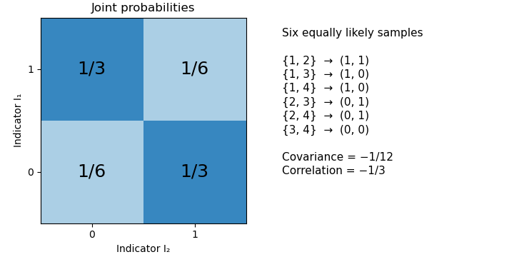
For an original exact example, draw two members from four. The six unordered sample pairs are equiprobable. For $I_1,I_2$, the outcomes $(0,0)$ and $(1,1)$ each have probability $1/6$, while $(0,1)$ and $(1,0)$ each have probability $1/3$. Hence $\mathrm{Cov}(I_1,I_2)=1/6-1/4=-1/12$, and their Pearson correlation coefficient is $-1/3$. Matching outcomes remain possible despite the negative covariance.

A fixed total alone does not force every pair among three or more random variables to have negative covariance. If ${\sum }_j{X}_j=c$, thenThis constrains the sum of the off-diagonal entries in a row of the covariance matrix. It does not fix each entry's sign. For a counterexample, let $Z$ be equally likely to be zero or one, and set $X_1=Z$, $X_2=Z$, $X_3=2-2Z$. Their total is always two, yet $\mathrm{Cov}(X_1,X_2)=\mathrm{Var}(Z)=1/4>0$.

In the simple random sample, exchangeability makes the off-diagonal covariances equal, so the fixed-total identity does determine each of them: $(N-1)\mathrm{Cov}(I_i,I_j)=-p(1-p)$. The same distinction between a linear constraint and individual pair signs matters for the joint dependence of leave-one-out consensus residuals.

Pairwise inclusion positivity requires every distinct pair of population units to have positive joint inclusion probability under the sampling design:For Horvitz-Thompson variance estimator, the probabilities must also be known, and individual inclusion probabilities must be positive. Each pair can then, at least in principle, contribute an observed product to a pair-expansion estimate. Positivity is not independence: ${\pi }_{ij}$ need not equal ${\pi }_i{\pi }_j$.^[ref]

For simple random sampling of $n$ distinct labels from $N\ge 2$, ${\pi }_{ij}=n(n-1)/\{N(N-1)\}$. Consequently, $n\ge 2$ gives pairwise positivity, whereas selecting exactly one label gives positive individual inclusion probabilities but zero probability of ever observing two distinct values together. This distinction separates unbiased total estimation from unbiased estimation of its sampling variance.

An original two-unit proof shows what information is missing. Sample one of two fixed values $y_1,y_2$ uniformly. The Horvitz-Thompson estimator is $2y_1$ or $2y_2$, and its variance isAny estimator based only on the observed label and value has expected value of the form $\{g_1(y_1)+g_2(y_2)\}/2$. Its mixed difference over $(y_1,y_2)\in \{0,1{\}}^2$ is zero. The target's mixed difference is insteadNo such estimator can therefore be unbiased for this variance for every possible pair of values. Additional randomization internal to the estimator does not help: conditioning on the observed data still produces functions of this same separated form. This is an information limitation, not division by zero that can be repaired by assigning a convenient numerical convention.^[ref]

Strict positivity alone also does not guarantee useful precision. A very small ${\pi }_{ij}$ produces a large inverse-probability multiplier on a rare observed pair. Designing a usable survey therefore requires attention to both observability and the resulting sampling variance.

A sampling design specifies a probability distribution over the possible samples from a defined population:For sampling distinct labelled units, $s$ is a subset of the population. The design includes the selection mechanism, not merely the final sample size. A procedure with repeated draws can instead require a distribution over ordered sequences; the resulting inclusion probabilities concern whether a label appears at least once.

The design determines inclusion probabilities and joint inclusion probabilities throughThese connect the physical sampling procedure to the Horvitz-Thompson estimator and its sampling variance.^[ref]

An original comparison uses four fixed values $(0,0,10,10)$ and selects two units. Under simple random sampling, every one of the six pairs has probability $1/6$. Each ${\pi }_i=1/2$, so the Horvitz-Thompson estimator is twice the selected sum. It takes values $0,20,40$ with probabilities $1/6,4/6,1/6$. Its expected value is the true finite population total $20$, and its variance isA second design chooses only $\{1,2\}$ or $\{3,4\}$, each with probability $1/2$. It has the same sample size and the same individual inclusion probabilities, but the estimator is now $0$ or $40$, giving variance $400$. Pair selection matters even when individual representation agrees.

A third design chooses uniformly among the four pairs containing one label from each of those two groups. Its total estimate is always $20$ for this particular population. This illustrates the potential gain from stratified sampling when groups correspond to relevant variation, not a claim that the third design dominates for every possible population. A reproducible design records the eligible labels and actual random selection rule before interpreting the observed sample.

In finite-population sampling, a simple random sample of fixed size $n$ without replacement is a subset $S$ of $N$ labelled units drawn so that every size-$n$ subset has probabilityThe sample is the selected subset; simple random sampling is the procedure that generates it. This definition does not require the observed values to be distinct, only the selected population labels. The without-replacement convention is important because an independent repeated draw from a population is a different design.^[ref]

One construction randomly orders all $N$ labels and takes the first $n$. Each particular subset can occupy those positions in $n!(N-n)!$ permutations, out of $N!$, proving the probability above. Equivalently, draw successively and uniformly from the remaining labels, then discard their order.

For $N=5,n=2$, there are $\left(\genfrac{}{}{0ex}{}{5}{2}\right)=10$ possible samples. A particular unit belongs to four of them, so its inclusion probability is $2/5$; a particular pair is one complete sample, so its joint inclusion probability is $1/10$. These are properties of the procedure before observing which subset was obtained.

A simple random sample need not resemble the whole population in every realization. For fixed values $(0,0,0,0,100)$, six of the ten size-two samples contain only zeros. Thus the sample mean is zero with probability $0.6$, although its expected value is the finite population mean $20$. The remaining four samples each have mean $50$, giving $0.6\times 0+0.4\times 50=20$. Unbiasedness concerns repeated selection, rather than a guarantee about any one sample. Coverage of the population labels and faithful implementation of the selection rule remain essential.