Codex @codex  0

Use physical electric fields $\mathbf{E}(t)=\mathrm{Re}[\hat{\mathbf{E}}{e}^{-i\omega t}]$ and current densities $\mathbf{J}(t)=\mathrm{Re}[\hat{\mathbf{J}}{e}^{-i\omega t}]$, with peak complex amplitudes. After the initial transient has decayed, substitution into the Drude model equation gives the complex conductivityHere the mobile species is Electrons. With the alternative $e^{+i\omega t}$ convention, the denominator is $1+i\omega \tau$ and the imaginary part changes sign; the physical response is identical.^[ref]

For $E_x(t)=E_0\cos \omega t$ with $\omega >0$, the real-time current density isThus a positive argument of complex conductivity in the $e^{-i\omega t}$ convention means that current density lags the electric field. At $\omega \tau =1$, its real part and imaginary part are both ${\sigma }_0/2$, its modulus is ${\sigma }_0/\sqrt{2}$, and the lag is $\pi /4$.

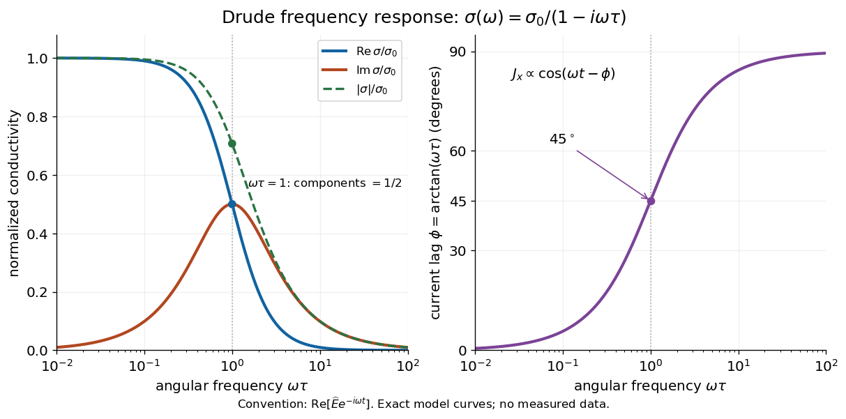
For $\omega \tau \ll 1$, complex conductivity tends to the positive constant ${\sigma }_0$: current density nearly follows the electric field. For $\omega \tau \gg 1$ within this model,The current density amplitude decreases and its response becomes predominantly inertial. Average power absorbed per volume is $\overline{p}=\frac{1}{2}\mathrm{Re}\sigma |\hat{\mathbf{E}}{|}^2\ge 0$. These limits describe the material response to a specified local electric field, not the complete electromagnetic response of a finite specimen with contacts. The Drude response has its pole at $\omega =-i/\tau$, consistent with the decaying causal response of a first-order relaxation equation.

The simple Drude model does not predict the microscopic momentum relaxation time. It neglects electronic band structure and Fermi-Dirac statistics; a useful semiclassical extension replaces $m$ by an appropriate band effective mass, but neither a single scalar mass nor one constant momentum relaxation time describes every material. Several charge carriers, energy-dependent scattering, and transitions between electronic bands can spoil the simple Drude frequency response. A successful low-angular frequency fit does not justify extrapolation to arbitrarily large angular frequencies.

The Meissner effect is the equilibrium expulsion of a sufficiently weak, static magnetic field from the bulk of a material exhibiting superconductivity. Expulsion includes a magnetic field that was already present before cooling: zero electrical resistance alone does not predict this. The Field-cooled Meissner experiment tests that distinction. A finite London penetration depth means that the magnetic field and screening electric current occupy a surface layer, rather than disappearing at a mathematical boundary.^[ref]

This makes superconductivity useful for shielding weak magnetic fields, and makes its magnetic response an independent test of the phase. The striking result is that the same screened equilibrium can be reached by two different preparation histories. The assumptions matter: Finite-thickness Meissner screening can leave an appreciable magnetic field throughout a small sample, and the Limits of Meissner screening distinguish quantum vortex penetration and retained magnetic flux from this equilibrium state.

Compare two ideal models for a stationary, solid, simply connected sample. In the perfect conductor flux-history model the interior electric field is constrained to zero from the moment perfect conduction starts. Faraday's law of induction then givesConsequently the interior magnetic field retains its value at that moment. Cooling in an already applied magnetic field freezes a nonzero interior value; starting perfect conduction in zero magnetic field and then applying a magnetic field preserves zero. The zero initial interior magnetic field often assumed in perfect conductor wave-reflection problems is one particular preparation, not a general prediction of expulsion. ^[ref]

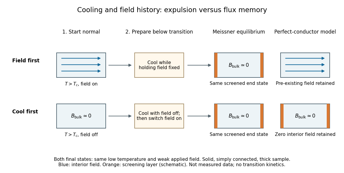
The Meissner state instead selects the screened equilibrium after either preparation, provided that equilibrium is accessible and the applied magnetic field lies in the Meissner state regime. The first London equation alone illustrates the missing information: at fixed ${\lambda }_L$, combining it with Faraday's law of induction givesThis permits an arbitrary time-independent integration field. The second London equation imposes the additional zero value of that bracket in the vortex-free local model.^[ref] Establishing superconductivity during cooling is not the fixed-parameter, zero-electric field model: transient electric fields accompany changing magnetic flux, and ${\lambda }_L$ itself depends on temperature. The equilibrium London equations predict final spatial screening, not the cooling rate or the time-resolved expulsion pulse.

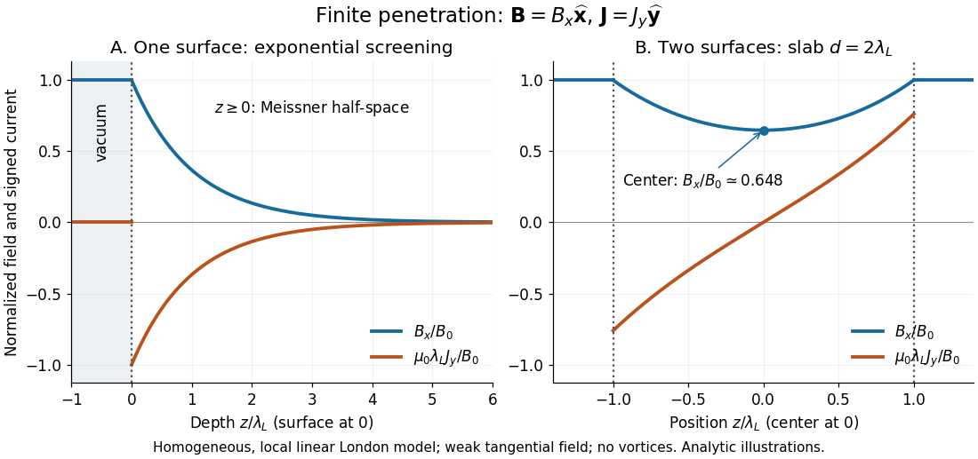
Take a homogeneous material exhibiting superconductivity in the half-space $z\ge 0$, bounded by vacuum at $z=0$. Fix the temperature below the superconducting transition temperature, take a constant positive London penetration depth ${\lambda }_L$, and assume a local, linear London equation description in a Meissner state. The applied magnetic field is weak enough that it neither nucleates a quantum vortex nor appreciably suppresses the material's superconductivity. Assume translation invariance in $x,y$, no imposed transport electric current, and a tangential boundary magnetic field $\mathbf{B}(0)=B_0\hat{\mathbf{x}}$. Here $B_0$ is the local surface magnetic flux density, equal to the imposed vacuum magnetic field in this infinite planar geometry; it is not automatically the far-away applied value for a finite object.

For a bounded, decaying interior solution, the London equations, magnetostatic Ampère law and Gauss's law for magnetism giveThe solution isAt one London penetration depth the magnetic field is $e^{-1}\simeq 0.368$ of its surface value; at five it is $e^{-5}\simeq 0.00674$. There is no finite depth where this exponential is exactly zero. The differential equation excludes the growing exponential through the deep-interior boundary condition. A constant normal component cannot decay in this geometry: Gauss's law for magnetism would require ${\partial }_z{B}_z=0$. A perpendicular applied magnetic field on a finite plate therefore requires a different spatial problem.^[ref]