Superconductivity is a phase of matter that supports steady electric current with zero bulk electrical resistivity and exhibits the Meissner effect: equilibrium screening of a sufficiently weak, static magnetic field from the interior. It occurs below a material-dependent superconducting transition temperature, provided the electric current and applied magnetic field are also sufficiently small. [ref]
https://arxiv.org/abs/cond-mat/0409402. Milind N. Kunchur (2004), limits on dissipation-free superconducting current
Bulk expulsion means that a sample much thicker than its London penetration depth has an almost field-free interior; the magnetic field need not vanish at its surface. Conventional BCS theory explains superconductivity through correlated electrons forming Cooper pairs. [ref]The two observations answer different questions. A resistance-versus-temperature experiment for superconductivity asks whether a steady electric current requires a measurable electric potential difference. A Field-cooled Meissner experiment asks whether a magnetic field already present in the material is expelled when it enters superconductivity. An ideal perfect conductor with zero electrical resistivity can preserve that pre-existing magnetic field; zero electrical resistance alone therefore does not establish the Meissner effect.
The usefulness follows directly from Joule heating, : maintaining a steady electric current through a segment with zero electrical resistance produces no resistive heating in that segment. This makes persistent electric currents attractive for producing steady magnetic fields. The beauty is that one phase has both a transport property and an equilibrium magnetic response, and the second cannot be inferred just by making an ordinary electrical resistance very small. The London equations encode this extra magnetic response. [ref]
https://doi.org/10.1098/rspa.1935.0048. F. and H. London (1935), The electromagnetic equations of the supraconductor
A change between normal and superconducting phases. Its existence gives a physical reason why an experimentally successful normal-state resistance model need not extrapolate through every lower temperature.
Superconducting pairing outside the simple conventional isotropic spin-singlet scenario, with the precise classification depending on the context and evidence. Gap symmetry, pairing mechanism, spin structure and time-reversal behavior are separate questions; a nonstandard gap does not establish every other proposed broken symmetry.
Pairing with d-wave orbital structure, such as a crystal gap proportional to . Its sign changes under a quarter-turn rotation, but a compensating overall phase change can leave gauge-invariant observables fourfold symmetric. Gap nodes and phase signs therefore do not by themselves establish nematicity or time-reversal breaking. A phase-sensitive test of d-wave pairing probes relative signs through interference.
Near clean two-dimensional d-wave nodes, linearized quasiparticle energies form anisotropic cones. Their low-energy density of states is proportional to , so electronic heat capacity scales as rather than the activated low-temperature form of a full gap. The clean in-plane penetration-depth increment is linear in T. Disorder, dimensional effects, vortex fields and gap changes can alter these laws, so the assumptions should accompany any proposed diagnostic.
Vortex superflow Doppler-shifts low-energy quasiparticles in a nodal superconductor. For a circular cell of radius and flow magnitude proportional to , its spatially averaged magnitude is proportional to . A linearly vanishing nodal density of states then acquires a zero-energy contribution proportional to , producing a low-temperature linear heat-capacity coefficient with that scaling. This is a clean semiclassical mixed-state estimate; the vector flow average can be zero, and disorder, screening, core states and other field effects change its range of validity.
For four equivalent nodes, two spin quasiparticles and local dispersion , one node encloses momentum area . Counting states with measure gives the displayed positive-excitation density. The associated clean low-temperature heat capacity is . Electron-addition spectral density alone has a different count because its coherence weights do not count all particle and hole thermal excitations.
A superconductor whose pairing order parameter has the angular or crystal-symmetry structure of d-wave superconductivity. The sign of the gap depends on momentum direction and nodes can permit low-energy fermionic Bogoliubov quasiparticles.
For nearest-neighbor spin-singlet pairing on a square lattice, opposite signs of the pairing amplitude on the two bond directions give the displayed momentum-dependent superconducting gap function. It changes sign under a quarter-turn and has nodes on the zone diagonals. This sign structure is distinct from a nonnegative gap whose magnitude is merely anisotropic. A real pure pattern does not by itself require broken time reversal.
An electromagnet whose winding uses a superconductor, allowing large currents without the normal winding's steady resistive loss in its superconducting state. Refrigeration, strain, field-dependent critical current and superconducting quench protection remain practical constraints. Magnetic resonance imaging, nuclear magnetic resonance and particle accelerators are applications.
A transition of part of a current-carrying superconducting system into a resistive state. Joule heating can spread the transition, and the stored magnetic energy must be handled safely by the system's protection design. Zero steady winding resistance does not remove the finite magnetic energy or the refrigeration requirement.
The condensation energy of a superconductor is the free-energy lowering on entering the superconducting state, with sign convention specified. For a local Landau density and , its minimum is relative to the normal-state value. The positive energy required to destroy the condensate is the opposite sign.
Coupling a charged condensate's phase to electromagnetism changes the neutral Goldstone response into electromagnetic collective dynamics. In a bulk long-wavelength regime, the longitudinal phase-density mode has a plasma gap. Its dispersion and damping require a dynamical model; a static Ginzburg-Landau functional alone does not fix the entire excitation spectrum.
A lossless low-energy charged-condensate action has a positive compressibility coefficient , effective pair density , mass and signed charge . Coupling its phase to the electromagnetic potentials through the displayed combinations preserves gauge symmetry. Adding the Maxwell action and eliminating the longitudinal electric potential gives in a simple homogeneous bulk model. Removing the electromagnetic coupling leaves neutral sound. Static Ginzburg-Landau theory of superconductivity alone cannot determine these frequencies or their damping. [ref]
Physics 215C: Quantum Field Theory, Part 3 by John McGreevy. §2.3, phase effective theory and coupling to electromagnetism
The superconducting intermetallic used in high-field conductors. Maintaining current-carrying connectivity and controlling strain are distinct from achieving a large upper critical field.
A superconducting alloy used in magnet conductors. Its useful critical current depends on flux pinning and processing as well as the equilibrium upper field.
A superconducting persistent current is an electric current circulating in a closed path with superconductivity after the external driving electromotive force has ceased. Its associated magnetic field makes the circulation observable without inserting a measuring instrument into the path. This article concerns macroscopic circulation in superconductivity. A finite experiment establishes persistence over its observation window with a stated measurement error, rather than directly observing an infinite lifetime.
The ideal circuit connection is flux conservation in a superconducting loop. In a fixed loop with self-inductance , a single circulating electric current , and externally imposed linked magnetic flux , the lumped circuit approximation givesWhen the electrical resistance vanishes, integrating gives . Removing the external linked magnetic flux therefore changes the circulating electric current; holding it fixed afterwards preserves that electric current. This is a circuit approximation with a specified self-inductance, not a derivation of the microscopic state of superconductivity. For thin paths where the carrier contribution matters, fluxoid and flux quantization in a superconductor supplies the more careful description.
For constant , constant effective electrical resistance , and no changing external linked magnetic flux, the RL circuit instead predictsThis exponential decay follows by separating . A long relaxation time tests extremely small electrical resistance without trying to resolve an equally tiny steady electric potential difference. The stored magnetic energy is , so the same model gives , exactly the Joule heating loss. The finite energy stored in the loop supplies the magnetic readout; the circulating electric current is not a continuously powered source of useful work.
The persistent current in a superconducting loop experiment prepares a closed cold path, changes the externally linked magnetic flux, and follows the resulting superconducting persistent current through its magnetic field. The essential measurement starts after the inducing magnetic field has stopped changing.
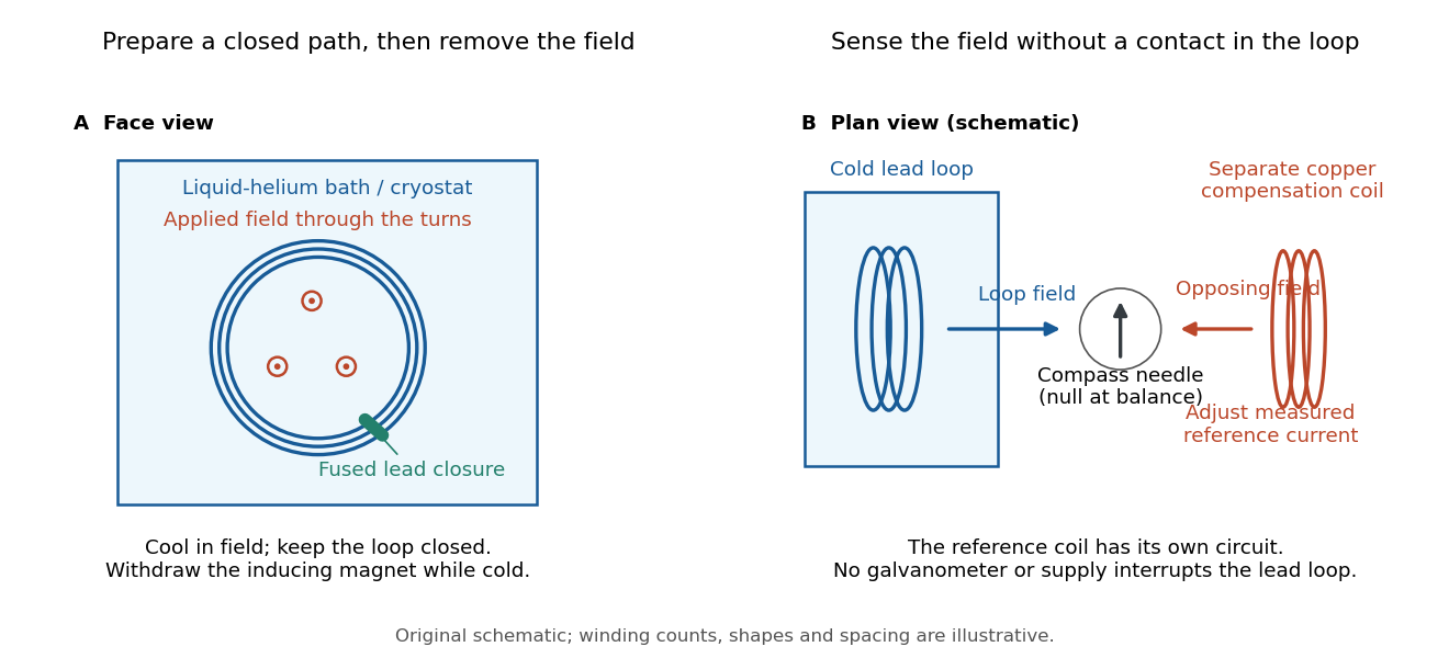
Heike Kamerlingh Onnes's 1914 Communication 140c describes a lead coil closed by fused lead connections. Cooling in a magnetic field and removing the inducing magnet prepared the circulation. A magnetic compass sensed it without contacts; a separate copper coil, cooled in liquid air, supplied a measured balancing magnetic field. Reversing orientation and compensation reduced offsets. [ref]
Further Experiments with Liquid Helium, J (Continued) by Heike Kamerlingh Onnes. Communication 140c (1914), §5, pp. 278–280; §7, pp. 280–281
The liquid-helium cryostat maintained low temperature, but refilling temporarily warmed the apparatus and changed the inferred electric current. A later run used a smaller initial electric current. Apparatus deformation and needle-zero drift limited comparison; cutting the closure still left a smaller magnetic signal, warning against assigning every signal to circulation around the whole loop. The report consequently gave an upper bound under a residual Ohm's law hypothesis. [ref]
Further Experiments with Liquid Helium, J (Continued) by Heike Kamerlingh Onnes. Communication 140c, §5, pp. 279–280; §6, p. 280; §8, pp. 281–283
For interpreting such a measurement, write a locally calibrated magnetic signal asHere is the coupling and gain, while contains the background magnetic field and readout offset. Only after establishing stable and correcting does a ratio of signals determine a ratio of electric currents. A gradual change in geometry, a drifting background magnetic field, or a change of temperature can imitate or conceal a decay. A pickup coil connected only to a voltage meter obeys Faraday's law of induction and detects a changing linked magnetic flux; its zero steady output cannot demonstrate that the underlying static magnetic field has disappeared. A magnetic compass can respond to that static magnetic field.
Opening the path, reversing the preparation, and repeating with smaller initial electric current are useful controls for separating whole-loop circulation, magnetic background and a superconducting critical current. Keep the temperature and external magnetic field stable during the interval used to infer electrical resistance. A sudden reduction near a superconducting critical current is not evidence for the constant- exponential decay model at smaller electric current. Persistence also does not replace the Field-cooled Meissner experiment: transport around a hole and magnetic expulsion from the material test different properties.
Suppose a calibrated measurement bounds the fractional loss of a nonzero superconducting persistent current by , with , over a duration . Take by choosing the circulation direction. Under the constant-, constant-, undriven RL circuit model,The inequality follows because the logarithm is increasing. The final approximation requires and slightly understates the exact upper bound. If is uncertain, an independently established upper bound on gives the conservative electrical resistance bound. The uncertainty in the initial reading, the final reading, background subtraction and drift must all be included in ; a display resolution alone does not provide it.
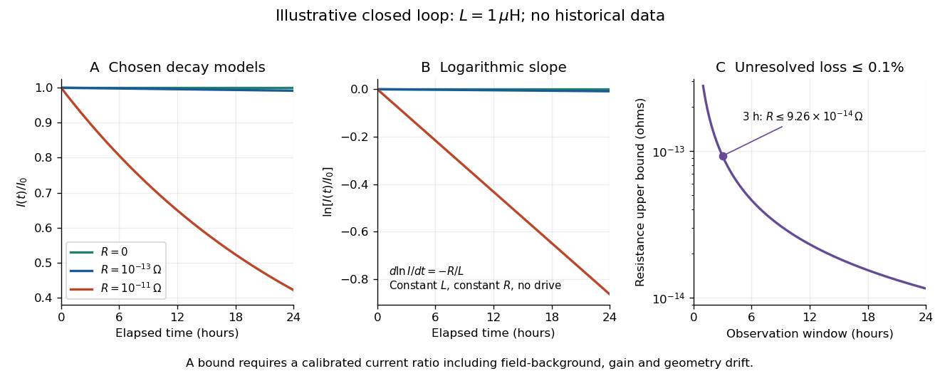
An illustrative exponential decay, its logarithmic slope and the resulting resistance bound
. Chosen numerical model, not historical data: fixed self-inductance and no external drive. The final panel assumes a calibrated fractional-loss bound of at each chosen observation duration. Longer observation tightens the bound only while that fractional uncertainty remains controlled. Details.For an original illustrative example, let and suppose the corrected electric current ratio after is at least . ThenThese are conditional bounds for stipulated parameters, not values attributed to the 1914 apparatus. With the same but , the model instead gives and : a readily visible loss on the chosen scale.
A resolved decay can be checked using its logarithm:A straight line supports this constant-parameter model; curvature or jumps demand a different account. If an effective electrical resistance varies with time while remains fixed and the loop remains undriven, only its time average is constrained:This does not bound every instantaneous value of . Changing self-inductance or external linked magnetic flux adds terms to the circuit equation, so an uncorrected magnetic signal cannot simply be substituted for . Nonobservation of decay leaves arbitrarily small positive constant electrical resistance compatible with a finite observation: it is not a logical proof that .
A superconducting critical current is the limiting electric current, for a specified sample, temperature, external magnetic field and measurement criterion, beyond which the chosen state of superconductivity no longer sustains dissipation-free transport. A weak connection can limit a loop before the rest of its material does. A magnetic field generated by the electric current itself also contributes to the sample's conditions. A limit on the initial superconducting persistent current and a bound on its subsequent electrical resistance answer different experimental questions.
A limiting transport current per conductor cross-sectional area for specified temperature, magnetic field and dissipation criterion. Local current distribution, flux motion and weak links can make it distinct from an intrinsic depairing limit. Its variation with the operating conditions is summarized by a superconducting critical surface.
For uniform flow in local Ginzburg-Landau theory of superconductivity, a phase gradient suppresses the equilibrium condensate density by . Hence , maximized at . This intrinsic local limit differs from vortex entry, depinning and the cross-section average in a thick wire. A Meissner surface shell has average-to-surface current-density ratio approximately for wire radius .
The boundary of a stated superconducting transport criterion in temperature, magnetic field and current-density space. A value measured under one combination does not specify a winding's usable current at another field or temperature. Strain and sample geometry can require further parameters.
A type-II superconductor can admit magnetic flux through quantized vortices while retaining superconductivity between their cores. Its superconducting mixed state lies between the lower critical magnetic field and upper critical magnetic field. These are equilibrium bulk distinctions; sample shape, flux pinning and preparation affect a measured magnetic response.
The motivating thin-film experiments changed an apparently minor preparation detail. Nikolay Zavaritskii evaporated metal onto glass; Alexander Shalnikov proposed cooling the substrate to helium temperatures to suppress agglomeration. The resulting critical-field behavior no longer matched the small-parameter approximation. Alexei Alexeyevich Abrikosov found a different regime within the same theory, rather than discarding its equations.[ref]
Nobel Lecture: Type-II superconductors and the vortex lattice by Alexei Alexeyevich Abrikosov. p.975, film preparation and the second group
An Abrikosov vortex has a core where the superconducting order parameter is suppressed, surrounding circulating electric currents, and a winding of its quantum phase. A singly wound vortex carries one superconducting flux quantum in the appropriate bulk flux-quantization limit. The exact contour statement is fluxoid and flux quantization in a superconductor; the enclosed magnetic flux alone need not equal a flux quantum on a contour with appreciable electric current.
A periodic array of Abrikosov vortices. In the isotropic local theory near the upper critical magnetic field, the triangular array has a lower Helmholtz free energy than the square array.[ref]
Nobel Lecture: Type-II superconductors and the vortex lattice by Alexei Alexeyevich Abrikosov. p.976, equations3–4 and the two lattice geometries
The useful distinction is between vortex existence, array geometry, and vortex mobility. Quantized winding does not force every array to be triangular or defect-free. A stationary array and vortices moving under an applied electric current also have different transport consequences; flux pinning matters for carrying useful electric currents.
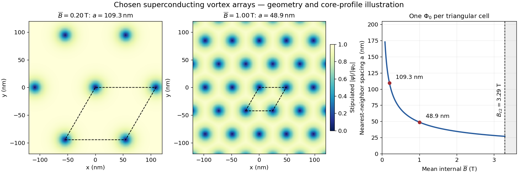
Assume a triangular array of straight, singly quantized Abrikosov vortices with nearest-neighbor distance . Here is the magnitude of the spatially averaged internal magnetic field, and is the superconducting flux quantum; is the elementary charge. Two lattice vectors of length meeting at span area . One flux quantum per cell givesThus multiplying by five decreases by ; it does not multiply the flux of each vortex by five. Using the exact SI Planck constant and elementary charge, .[ref]
For chosen internal fields and , the spacings are approximately and . These are geometric model calculations, not measurements from a particular sample. The local magnetic field varies within a cell; replacing by the field at a core would not give this counting relation.
A measure of spatial nonuniformity in the order parameter, with averages taken over one lattice cell. Set . ThenEquality requires uniform , so a nonconstant core pattern costs more in the quartic term than a uniform amplitude with the same mean squared amplitude. This identity alone does not compare two different vortex arrays: their admissible profiles must also satisfy the field equations.
U. Essmann and H. Träuble reported triangular vortex arrays, including defects, using electron microscopy on lead-indium and niobium samples in the remanent state.[ref]
The direct observation of individual flux lines in type II superconductors by U. Essmann and H. Träuble. Publisher abstract, materials, electron microscopy and remanent-state lattices
Such a prepared state need not display the equilibrium array at a uniform applied field. Images of regular positions and a proof of unrestricted vortex motion would answer different questions.Slow motion of pinned superconducting vortices, commonly through thermally activated escape over energy barriers. It permits magnetic relaxation and a small dissipative voltage even below an ideal static depinning force. The barrier depends on current and pinning structure; a universal sharp transport threshold should not be assumed.
Motion of a previously pinned Abrikosov vortex when drive, thermal activation or other fluctuations overcome its trapping. The resulting flux motion can generate an electric field, so a transport critical current depends on the measurement's voltage and time criteria.
The superconducting transition temperature is the temperature at which the material enters superconductivity on cooling in zero applied magnetic field and with negligible measuring electric current. A measured transition at nonzero magnetic field or appreciable electric current need not occur at this zero-field . If a resistance-versus-temperature experiment for superconductivity gives a transition spread over several temperatures, report whether its quoted value is the onset, midpoint, or disappearance of detectable electrical resistance, together with the experimental conditions. This operational distinction matters when comparing samples. [ref]
Pairing can establish a local binding or gap scale before a system develops phase-coherent transport. An actual superconducting transition temperature depends on both the pair scale and the phase stiffness. Low carrier density or weak interlayer coupling can make phase ordering the lower scale even when the pairing amplitude is appreciable. A minimum or smooth interpolation of two estimated scales is a qualitative guide, not a substitute for a self-consistent theory of the crossover.
The motivating observation is an abrupt disappearance of detectable electrical resistance on cooling, rather than a smooth improvement in conduction. The diagram pairs the measuring arrangement with an idealized transition. Its curves are deliberately synthetic; neither their scales nor their abrupt step are a reconstruction of measured mercury data.
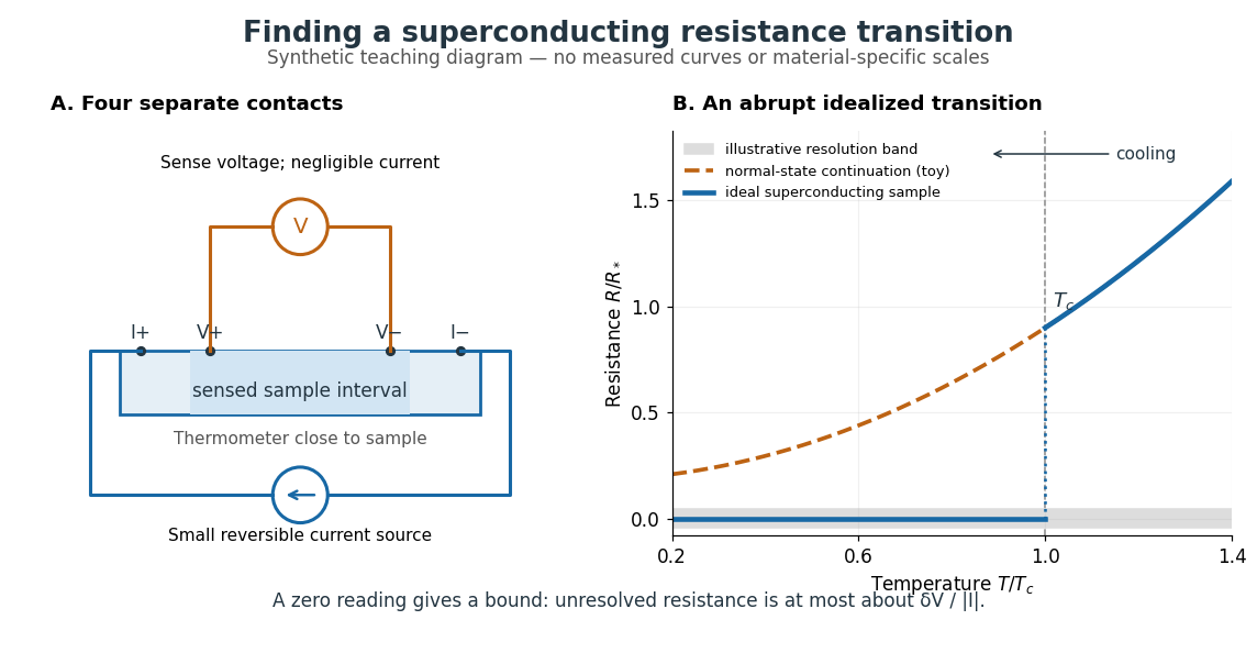
In a report communicated in November 1911, Heike Kamerlingh Onnes described a mercury thread in seven connected glass U-tubes immersed in a stirred liquid-helium bath. Expansion spaces kept freezing mercury from breaking the glass or interrupting the thread. Separate leads supplied electric current and sensed electric potential difference. He compensated a troublesome thermoelectric effect and reversed the main electric current to extract the resistive signal. He reported a rapid fall between and on his stated historical temperature scale, with electrical resistance disappearing at the lower value. The apparatus and control of spurious electric potential differences are part of the discovery, not incidental details. [ref]
https://dwc.knaw.nl/DL/publications/PU00013242.pdf. Kamerlingh Onnes, Communication 124c (1911), §§2–3, pp. 819–821
A modern version places a contacted sample and a calibrated thermometer close together in a cooling environment. Use four-terminal sensing, record the small applied electric current , the sensed electric potential difference , and the sample temperature , then plot . Repeat on warming as well as cooling, and allow readings to stabilize near thermal equilibrium. Disagreement between warming and cooling is a reason to check sample–thermometer lag and reproducibility before quoting a superconducting transition temperature. Mikhailov and Kordosky's undergraduate experiment uses this strategy with liquid-nitrogen cooling. [ref]
https://physics.wm.edu/~evmik/classes/2021_fall_Experimental_Atomic_Physics_251/lab_descriptions/superconductivity/. Mikhailov and Kordosky, Physics 251 superconductivity lab, measurement procedure and discussion
Choose the measuring electric current small enough that Joule heating does not appreciably change the sample temperature, and repeat with a smaller electric current to check that the transition persists. Cancel stable offsets using the reversal described in four-terminal sensing. A reading indistinguishable from zero supplies an experimental upper bound, not a proof of exact zero electrical resistance. If bounds the unresolved resistive electric potential difference, thenFor a stipulated sensitivity and , this is . The bound applies between the sensing contacts; it is not the electrical resistance of the complete wiring. A conducting path through part of an inhomogeneous sample can also make negligible, so the Field-cooled Meissner experiment adds independent evidence about the material's magnetic response.
Four-terminal sensing uses one pair of contacts to carry electric current and a separate pair to sense electric potential difference. The sensing instrument draws negligible electric current, so the voltage drops along its own leads are negligible, and the current-contact drops outside the sensing interval are excluded. A measurement using just two shared leads includes their electrical resistance and contact drops, which can overwhelm the small sample signal in a resistance-versus-temperature experiment for superconductivity. Four contacts do not automatically remove offsets from the thermoelectric effect. [ref]
https://www.tek.com/en/documents/technical-article/low-voltage-measurement-techniques. Tektronix, Low-Voltage Measurement Techniques, four-lead arrangement and thermoelectric offsets
For a stable offset , let denote the magnitude of the reversed electric current. The measured electric potential differences are and , so subtraction gives the displayed electrical resistance. For example, with stipulated , and , the two readings are and ; their difference correctly recovers . If the offset changes between readings, its change leaves a residual measurement error; the sample and measuring circuit must remain sufficiently stable during reversal.
The Field-cooled Meissner experiment starts above the superconducting transition temperature with a weak, steady applied magnetic field already penetrating a solid sample. Cooling while keeping the applied magnetic field fixed tests whether the interior magnetic flux changes. This is the decisive contrast with cooling in zero magnetic field and switching the magnetic field on afterwards. The diagram shows the two histories for the same final applied magnetic field.
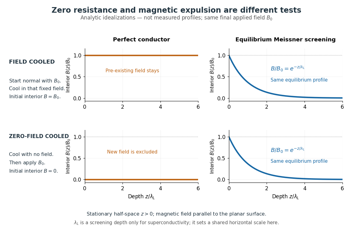
Meissner and Ochsenfeld reported magnetic expulsion in 1933, showing that the transition involves more than vanishing electrical resistance. A modern motivating version appears in MIT's lead-sample experiment: surround the sample with a solenoid supplying a steady magnetic field and a separate pickup coil connected to a recording instrument. Apply the magnetic field while the lead is still normal, then cool through its transition without changing the solenoid electric current. Expulsion produces a transient pickup-coil electric potential difference; warming through the transition produces the opposite sign as magnetic flux returns. MIT also checks the signal direction by switching off the applied magnetic field while the sample is normal. [ref]
https://hoffman.physics.harvard.edu/materials/SCintro.php. Hoffman laboratory, magnetic-expulsion discovery
[ref]Faraday's law of induction explains the readout. For a stationary -turn pickup coil, with the same linked magnetic flux per turn and a fixed orientation,Thus a transient measures a change in linked magnetic flux, not directly the static magnetic field at every point in the sample. For stipulated and per turn, the signed pulse area is . The apparatus geometry determines how a change in interior magnetic field contributes to that linked magnetic flux. Keeping the applied magnetic field fixed, repeating on warming, and checking a normal-state control make the expulsion interpretation testable; a stationary pickup coil has no sustained signal after the magnetic flux has stopped changing.
Why does the preparation history matter? In the stationary, ideal perfect conductor model, the interior electric field is zero. The differential form of Faraday's law of induction then givesIf the interior magnetic field was when perfect conduction began, it remains ; if it was zero, it stays zero when an external magnetic field is subsequently applied. Both a perfect conductor prepared in zero magnetic field and a sample exhibiting the Meissner effect can therefore exclude a newly applied weak magnetic field. Only the field-cooled comparison tests expulsion of an already present magnetic field. This argument concerns a stationary sample and the ideal zero-electric field model, not a moving conductor.
The equilibrium London equations supply the additional constraint. In a homogeneous region without penetrating flux tubes, they imply . For a half-space with a magnetic field parallel to its flat boundary, fixed surface value , and a bounded solution deep inside, this givesAt only of the surface magnetic field remains. The screening electric currents near the surface produce this reduction. Unlike the frozen interior magnetic field of a perfect conductor, this equilibrium profile does not retain an arbitrary initial . The extra constitutive relation, and not zero electrical resistance by itself, selects the screened state. Expulsion occurs during the transition, when transient electric fields can be present; the steady-state zero-electric field argument does not describe the process of establishing superconductivity. The diagram gives equilibrium end states, not transition kinetics. [ref]
https://doi.org/10.1098/rspa.1935.0048. F. and H. London (1935), magnetic screening beyond the acceleration equation
These ideal comparisons concern a solid sample in equilibrium and a sufficiently weak magnetic field. Stronger magnetic fields can destroy superconductivity or permit magnetic flux to penetrate parts of a sample, so complete bulk expulsion is not a claim about every superconducting state. [ref]
https://www.ocw.mit.edu/courses/6-763-applied-superconductivity-fall-2005/41b2882232b1b43823ec488969c21b6d_lecture1.pdf#page=6. Terry P. Orlando, Applied Superconductivity, Lecture 1 (2005), mixed-state magnetic penetration
A hole in a superconducting loop can retain magnetic flux even while the material surrounding it screens its own interior; see flux conservation in a superconducting loop. The hole is not superconducting material, so its retained magnetic flux does not contradict the Meissner effect. [ref]https://www.feynmanlectures.caltech.edu/III_21.html#Ch21-S7. Feynman, Leighton and Sands, III.21.7: field cooling a superconducting ring
Vitaly Lazarevich Ginzburg and Lev Landau applied an order parameter description to superconductivity in 1950. A spatially varying complex amplitude extends the fixed-amplitude description of the London equations. Their initial charge assumption preceded the later identification of the universal pair charge.[ref]
Consider the following isotropic, local SI Helmholtz free energy model near a continuous superconducting transition temperature:Here , is a phenomenological mass parameter, and fixes the electron-pair convention. The uniform superconducting minimum for has . The gradient term penalizes changes of the amplitude and the gauge-invariant quantum phase; the magnetic term penalizes magnetic field penetration. The gauge-coupling sign in Ginzburg-Landau superconductivity keeps the electric current and field equation consistent. This model omits material anisotropy, microscopic nonlocality and critical fluctuations.
A phenomenological near-transition relaxation equation for a charged complex order parameter, with a positive real relaxation coefficient in its simplest dissipative form. Under , and , the displayed time derivative transforms covariantly, as does the spatial derivative in the Ginzburg-Landau theory of superconductivity. Microscopic applicability depends on regime and scattering processes; this equation is distinct from a universal conservative condensate wave equation.
Expanding the BCS theory near the transition in small pair amplitude and slow spatial gradients produces a local complex order-parameter free energy. The microscopic theory fixes its normalization and coefficients, including the pair's twice-electron charge. This establishes a controlled near-transition relation rather than an exact all-temperature replacement for BCS theory.[ref]
Microscopic Derivation of the Ginzburg-Landau Equations in the Theory of Superconductivity by Lev Gor'kov. 1959 abstract and near-transition reduction
A pairing-channel Hubbard–Stratonovich transformation replaces an attractive fermion interaction by a complex Cooper pair field coupled to fermion pairs. A Grassmann Gaussian integral then gives a trace-log effective action, with its trace convention fixed to avoid doubling independent spin-pair blocks. The uniform stationary equation is the BCS gap equation. A small-field, slow-gradient expansion near the transition yields Ginzburg-Landau theory of superconductivity; the normalization of the phenomenological field need not equal that of the microscopic gap.
For a clean isotropic three-dimensional weak-coupling s-wave model, use the energy-valued gap , a density of states per spin, and free-energy density . Near , . The quartic coefficient follows fromThe integral is and the positive odd-integer sum is , yielding the displayed coefficient. The isotropic Fermi-velocity average gives . The pair charge is in . These values change under a rescaling of , different density-of-states convention or different material model; the local expansion is a near-transition approximation.[ref]
Microscopic Derivation of the Ginzburg-Landau Equations in the Theory of Superconductivity by Lev Gor'kov. Microscopic near-transition expansion; pair charge
The gradient and quadratic terms of the stated model balance at the amplitude-variation scale . It is a superconducting length scale, distinct from optical coherence length. The weak-field London penetration depth in the same normalization obeysA core suppresses the pairing amplitude over a scale set by ; screening electric currents and the magnetic field involve . Neither scale is a universal particle size.
In the isotropic single-component model, gives the type-I regime and the type-II regime; the interface-energy distinction belongs to the model, rather than a purely geometric test of core overlap.[ref]
Nobel Lecture: Type-II superconductors and the vortex lattice by Alexei Alexeyevich Abrikosov. p.975, interface energy and the type-II regime
Combining and gives . Its derivative is : the ratio peaks at , with maximum . Thus each has two solutions with . The large- branch is the one consistent with using a leading-log approximation; the small branch cannot be selected or rejected by the inequality alone. Omitted core-energy terms limit numerical accuracy.
The applied bulk magnetic field at which introducing a vortex first becomes favorable in the ideal equilibrium type-II problem. Surface barriers, sample shape and flux pinning can change the apparent entry field.
Linearize the stated model about in a uniform magnetic field. The kinetic operator has the Landau level ground energy . Its cancellation with givesThis is the bulk orbital field scale of this model; it excludes spin-polarization limits and uses the normal-state relation . For the chosen , it is about . With , . Counting triangular cells at would give , but it is the linearized field equation, rather than disks of an arbitrarily chosen core radius touching, that supplied the transition criterion.
For energy with kinetic term , , variation gives and current . Thus changing the sign of the covariant derivative changes the phase-gradient term of the current. The displayed energy, field equation and current must use the same convention.
A pair field transforms as when . Its phase gradient alone is gauge dependent; is invariant. With , the temporal combination is also invariant. The supercurrent is . A negative electronic pair charge is consistent with either sign of current once this convention is retained throughout.
A Josephson junction couples two regions with superconductivity through a weak link. A tunnel barrier is one implementation.
The remarkable possibility is a steady electric current across an insulating barrier at zero electric potential difference. This is the DC Josephson effect, carried by coherent transfer of Cooper pairs. It differs from single-electron superconducting tunneling, which probes the quasiparticle excitation spectrum and produces a dissipative current-voltage characteristic. Both contributions can occur in the same superconducting tunnel device. Brian D. Josephson predicted the pair contribution in 1962; his paper treats transfer that leaves the quasiparticle distribution unchanged. [ref]
Possible new effects in superconductive tunnelling by Brian D. Josephson. Josephson (1962), pp. 251–252, opening paragraph and equation (3)
The Josephson effect turns a difference of quantum phases into a measurable electric current, and an applied electric potential difference into a rate of phase advance. The Giaever gap experiment instead turns an electric potential difference into an excitation energy scale. These complementary measurements expose two aspects of superconductivity: its coherent order parameter and its gapped quasiparticle spectrum. The microscopic pairing calculation belongs to BCS theory and the BCS gap equation. A tunnel diode uses a different device, a semiconductor p-n junction.
Adding capacitance and an external bias makes the Gauge-invariant Josephson phase dynamical. Current-biased Josephson phase dynamics explains how its trapped energy levels and escape can be measured electrically.
A spatially uniform Josephson junction in a uniform transverse in-plane magnetic field has a linear gauge-invariant phase profile across its width. Integrating its sinusoidal local current-phase relation of a superconducting weak link gives a signed sinc coefficient multiplying the sine of the central phase. Maximizing over that phase gives the displayed nonnegative critical-current envelope. Zeros occur at nonzero integer multiples of the superconducting flux quantum. The relevant magnetic thickness includes electrode penetration when appreciable, and self-fields or nonuniform local critical current density alter the simple pattern.
A superconducting weak link is a connection between regions with superconductivity whose coupling is weak enough that a substantial difference of quantum phase can develop across the connection. An insulating tunnel barrier is one realization; a narrow conducting constriction can also couple the regions. The current-phase relation of a superconducting weak link depends on the connection. A sinusoid is the leading tunnel-junction approximation, not a universal law for every superconducting weak link. [ref]
The Discovery of Tunnelling Supercurrents by Brian D. Josephson. Josephson, Nobel lecture (12 December 1973), final discussion of weak links and tunnel barriers
The current-phase relation of a superconducting weak link gives its pair electric current as a function of the Gauge-invariant Josephson phase , at specified temperature and other conditions. For the ideal junction used below, with . More general periodic relations can contain higher Fourier harmonics; their maximum magnitude defines the corresponding superconducting critical current.
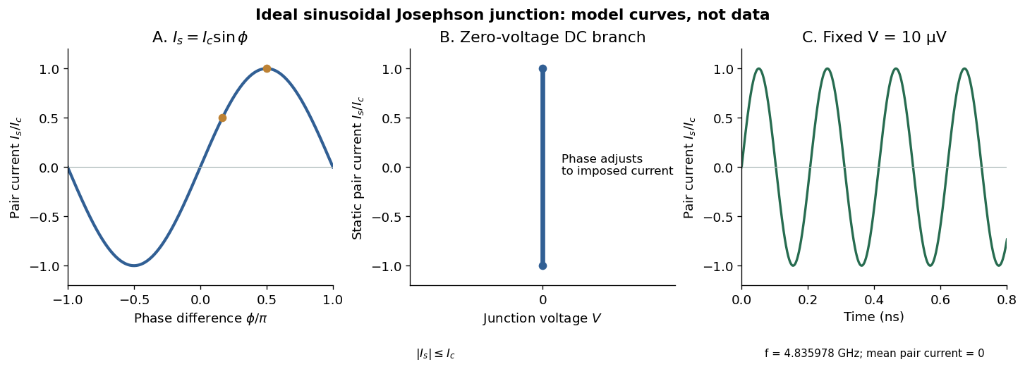
In the ideal sinusoidal Josephson junction, the pair electric current and quantum phase obeyHere is the magnitude of the electron electric charge, uses the Planck constant, and is the junction's superconducting critical current under the specified conditions. Define the signs as follows: positive conventional electric current flows from terminal 2 to terminal 1, and is the voltage of terminal 2 relative to terminal 1. The Gauge-invariant Josephson phase below fixes the matching orientation of . The DC Josephson effect and AC Josephson effect follow from these relations. [ref]
Possible new effects in superconductive tunnelling by Brian D. Josephson. Josephson (1962), p. 252, predictions (i) and (ii): zero-voltage supercurrent and frequency 2eV/h
A SQUID uses Josephson junctions in a loop made from a superconductor to detect changes in magnetic flux.
A superconducting loop containing one Josephson junction and coupled inductively to a radio-frequency resonator. Its flux-dependent nonlinear inductive response changes the resonator signal. A DC SQUID instead uses two junctions and can turn their critical-current interference into a voltage modulation under bias. Inductance, junction dynamics, noise and feedback determine the practical transfer function.
A SQUID with two Josephson junctions in a superconducting loop. For equal junctions, negligible self-inductance and no intrinsic phase offset, adding their sinusoidal currents gives the displayed flux-dependent critical current. An rf SQUID instead has one junction and uses loop inductance.
For an ideal symmetric two-junction interferometer with negligible self-flux, the stable zero-current phase is zero or pi according to the sign of the flux cosine. Linearization about that stable phase gives positive inductance. The stronger small-current condition is , and fails near a half-integer flux quantum where the ideal critical current vanishes.
The 1964 report established quantum interference in superconducting tunneling. It is an experimental counterpart to the phase-sensitive current predicted for coupled superconductors.[ref]
Quantum Interference Effects in Josephson Tunneling by R. C. Jaklevic and others. Primary experimental report, 1964
Write the superconducting order parameters as , using a field of pair electric charge . For a specified path across the superconducting weak link, defineHere is the magnetic vector potential. To check electromagnetic gauge invariance, use a scalar function and transformThe change of is , exactly cancelled by the change of the line integral. Thus is unchanged although each local quantum phase changes. This is the same charge/sign bookkeeping discussed in gauge-coupling sign in Ginzburg-Landau superconductivity. Different physical paths can enclose magnetic flux, so fixing the path matters.
For stationary reservoirs with equal internal pair chemical potentials and a time-independent vector potential, the local Schrödinger equation gives after dropping the common internal term. With electric potentials and , subtraction gives . For a general circuit, denotes the corresponding measured electrochemical voltage and the electromagnetic contribution must be treated consistently. A bare difference of phases without the vector potential term is insufficient in an arbitrary gauge.
The ideal Josephson junction has a phase-dependent energyDifferentiating and using the voltage–phase relation yieldsThus the ideal pair element stores and returns energy. At it carries a static electric current without electrical power loss. Under a nonzero periodic drive its instantaneous power need not vanish, but its energy returns after a full phase cycle. Real junctions also have a capacitance, quasiparticle transport and an external circuit; their total losses cannot be inferred from this conservative pair term alone.
At zero electric potential difference, permits a nonzero constant quantum phase and hence a steady pair electric current. Under an imposed electric current with , a static solution satisfies . The low-energy branch has . For example, a stipulated gives modulo ; it does not require a voltage drop. In the ideal current-biased energy , the positive second derivative on that branch explains its local stability.
The superconducting critical current is a maximum available static pair electric current, not the inevitable electric current under a voltage bias. At the initial state and circuit select a phase and a current. Above this sinusoidal model has no static phase solution, but its two relations alone do not predict the complete resistive current-voltage characteristic, switching dynamics or hysteresis. Those require the circuit and dissipative channels.
For constant nonzero voltage , direct integration givesA constant electric potential difference therefore produces an oscillating pair electric current. The average of this ideal sinusoid over a complete cycle is zero; a measured nonzero steady electric current can include single-electron superconducting tunneling. Josephson's lecture explicitly separates the ordinary quasiparticle term from the phase-dependent term. [ref]
The Discovery of Tunnelling Supercurrents by Brian D. Josephson. Josephson, Nobel lecture, discussion of I₀(V), the phase-dependent term and Fig. 2
For an original numerical example, use the exact SI values and . ThenThe corresponding period is about . These values describe an assumed exact applied voltage, not a historical measurement. The factor identifies coherent pair transfer; replacing it by would halve the predicted frequency.
A Josephson junction can make a collective quantum phase behave as a measurable dynamical coordinate. In current-biased Josephson phase dynamics, the Gauge-invariant Josephson phase moves in a tilted Josephson washboard potential; the junction's capacitance supplies its effective inertia. A trapped phase gives zero mean electric potential difference, while sustained phase advance produces a nonzero mean electric potential difference. Quantized phase levels in a Josephson junction and quantum escape of a current-biased Josephson junction test quantum mechanics for this collective coordinate.
Begin with a stipulated parallel electrical circuit: an ideal sinusoidal Josephson junction, capacitance , and effective electrical resistance . The Kirchhoff node law and Josephson effect giveHere is the constant bias electric current, is a deliberately applied microwave electric current, and represents unwanted fluctuating electric current. Multiplication by puts the undriven equation into the mechanical formThe effective inertia is a coefficient for a dimensionless quantum phase, not a literal material mass moving through the insulating layer. The capacitor's energy, , provides a direct check of that identification. The effective includes loading by the external electrical circuit; a constant parallel is an approximation over the relevant frequency range.
The useful design freedom is that changes the confinement while changes its inertia. The same manufactured device can therefore connect a classical oscillation, discrete energy levels, and escape to an electrical readout. The Martinis-Devoret-Clarke circuit experiments separate these questions experimentally. John Clarke, Michel H. Devoret and John M. Martinis shared the 2025 Nobel Prize in Physics for circuit experiments establishing macroscopic quantum tunnelling and discrete energy levels.[ref]
The Nobel Prize in Physics 2025 — Press release by Royal Swedish Academy of Sciences. 7 October 2025, p.1, award decision
At fixed positive bias ratio with , the Josephson coupling energy and work of the ideal bias source combine intoThis is the effective potential energy for an unwrapped Gauge-invariant Josephson phase; it includes the bias source and decreases by on advancing one period. A local minimum and the adjacent downhill barrier areTo verify the barrier, solve , select and , and subtract their potential energies. The small-oscillation angular frequency is fixed by the curvature:Thus the barrier and oscillation frequency both vanish as , but with different powers. For , expanding and givesThe first approximation is for a nearly critical bias. At the exact downhill barrier is ; at there is no confining local minimum in this model.
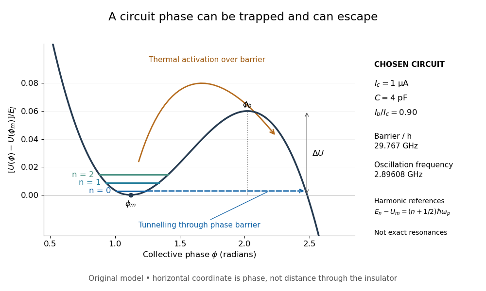
A tilted phase potential confines low energy levels and permits escape
. Original chosen model with , and . Three horizontal lines are quantum harmonic oscillator approximations , for ; they are not exact energy levels or measured data. The horizontal axis is a quantum phase, not distance through an insulator. Arrows distinguish over-barrier thermal activation and below-barrier quantum tunnelling. Details.For those stipulated parameters, direct evaluation gives , , and . Hence . The nearly critical barrier approximation gives , about below the exact result. These are original circuit calculations, not parameters assigned to the historical samples.
For a weakly damped well, quantizing the conservative part of current-biased Josephson phase dynamics gives the local Hamiltonian operatorThe tilted potential energy is unbounded downhill. Its trapped energy levels are therefore long-lived resonances with escape lifetimes, rather than globally bound stationary states. Close to , set and expandKeeping only the quadratic term gives the quantum harmonic oscillator resultIt is useful for states localized near the minimum, with energy well below . It does not count all the resonances accurately near escape. The omitted terms make successive spacings unequal. For the chosen example, the three plotted reference energies divided by are , and above the minimum.
A small microwave bias contributes . A one-photon transition between energy levels is resonant when . Exciting a higher energy level can strongly increase its escape probability. Measuring microwave absorption indirectly through escape therefore connects an invisible quantum phase state to a visible electric potential difference. A classical oscillation can also show resonance, so the mere existence of one peak is insufficient: the bias dependence and resolved unequal spacings are the discriminating predictions.
Quantum escape of a current-biased Josephson junction is decay of a trapped collective quantum phase state through a barrier in the tilted Josephson washboard potential. This barrier lies in the potential energy of an electrical circuit coordinate. Transfer of Cooper pairs across the physical insulating layer already supplies the Josephson coupling energy; it does not by itself demonstrate this further collective escape. Single-electron superconducting tunneling is a third, distinct process.
At higher temperature , thermal activation instead lifts the coordinate over the barrier. In the rare-escape regime its characteristic form is the Kramers escape ratewhere is the Boltzmann constant and the prefactor depends on damping and thermal equilibration. Cooling suppresses this route. For a quasistationary energy level at energy , the leading conservative WKB approximation instead haswith the two turning points bracketing the forbidden barrier. This is an exponential estimate requiring a large action compared with , slow escape compared with intrawell motion, and weak environmental corrections. It is not a complete rate prediction near the barrier top or with substantial damping.
The familiar cubic-barrier exponent can be checked independently. Choose , with . Its top is at and . At the well-bottom reference energy ,Substitution reduces the dimensionless integral to . This leading semiclassical action uses a cubic potential and a well-bottom reference; actual ground-state escape also needs the zero-point correction, prefactor and environment. In the chosen washboard example it gives after matching the exact barrier and curvature. This matching is an illustrative approximation, not an exact action integral for the cosine potential.
Escape need not yield a sustained voltage: the coordinate can become trapped again. The running-state readout assumes sufficient underdamping and bias to avoid such retrapping. The parallel model has quality factor ; large makes energy loss per oscillation small. Low-temperature rate saturation alone cannot distinguish quantum tunnelling from unwanted heating or external noise.
The 1985 spectroscopy experiment used niobium-based tunnel Josephson junctions on silicon, thermally anchored with final bias low-pass filters to a dilution refrigerator. Calibrated germanium and cobalt thermometers measured temperature. A filtered coaxial cable injected microwaves; repeated switches to nonzero electric potential difference measured escape with irradiation on and off. Bias scans at fixed microwave frequency resolved separate enhancements matching calculated unequal energy level spacings. Raising temperature merged the structure toward classical response. Junction parameters were calibrated in the classical regime; reducing the superconducting critical current with a magnetic field checked thermal readout. Parameter uncertainties limited absolute resonance positions.[ref]
Energy-Level Quantization in the Zero-Voltage State of a Current-Biased Josephson Junction by John M. Martinis and others. Original paper, pp.1543–1545, apparatus and Figs.2–4; p.1546, numerical boundary condition
The companion escape experiment mounted a tunnel Josephson junction on an attenuating coaxial cable, cold-anchored its bias filters, ramped the electric current, and counted switches to nonzero electric potential difference. Rapid current shutoff limited heating. Classical escape and microwave resonance calibrated the superconducting critical current, capacitance and environmental loading. Low-temperature escape agreed with the quantum prediction using these calibrated parameters. A magnetic field reduced the superconducting critical current to keep the same apparatus thermally activated at lower temperature, testing excess noise. Frequency-dependent loading contributed uncertainty; the predicted damping correction was smaller than combined errors, so the experiment did not resolve that correction.[ref]
Measurements of Macroscopic Quantum Tunneling out of the Zero-Voltage State of a Current-Biased Josephson Junction by Michel H. Devoret and others. Original paper, pp.1909–1910, calibration, Fig.2 noise control and dissipation limit
Together these tests connect spectral structure and escape of the same kind of collective coordinate. They do not constitute a demonstration of coherent gate operations on a qubit, or prove that every macroscopic coordinate retains quantum behavior under arbitrary environmental coupling. The attraction is more concrete: a fabricated electrical circuit admits both an independently measurable classical model and quantitative quantum tests of its phase dynamics.
A switching-current distribution of a Josephson junction records the bias electric current at the first detected transition to a sustained nonzero electric potential difference. Interpret it using a stipulated monotone ramp , a reproducible initial trapped state, and an instantaneous escape hazard function . Neglect retrapping and readout delay. The survival function obeys , so changing variable from time to electric current givesHere is a probability density function per unit electric current, not a rate per unit time. Division by the surviving population is essential: only trials still trapped can escape. A typical switching current is consequently not identical to the noiseless superconducting critical current.
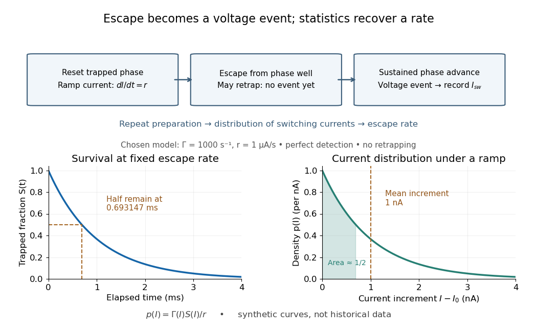
For an independent illustrative check, choose constant and . ThenHalf the trials have switched after , corresponding to of ramp. Doubling doubles the mean increment without changing the underlying escape rate. Real junction rates vary sharply with bias; this example isolates the statistical conversion.
Repeating the preparation, measuring the ramp, resolving the voltage onset, and allowing cooling after each dissipative event are prerequisites for this interpretation. Missed events, finite detection delay, changing temperature and retrapping alter the measured distribution. Even a correctly reconstructed rate needs the independent thermal and spectral checks before identifying its escape mechanism.
Single-electron superconducting tunneling transfers individual electrons across a barrier into or out of quasiparticle states of a material with superconductivity. In a normal-metal–insulator–superconductor junction, abbreviated NIS, only one electrode has superconductivity. Such a junction can reveal a superconducting energy gap without supporting a DC Josephson effect between two superconducting reservoirs.
For an elementary interpretation, assume an opaque barrier, approximately constant normal-electrode density of states, and an energy-independent tunneling matrix element over the range probed. Write the superconducting density of states divided by its normal-state value as , with measured from its chemical potential. A signed voltage convention chosen for positive normal-electrode injection giveswhere is the Fermi-Dirac distribution at a common temperature and is the normal-state junction electrical resistance. This current convention is local to the NIS measurement. The expression counts occupied initial and empty final states; it is a quasiparticle transport model, not a current-phase relation of a superconducting weak link.
An original analytic illustration uses the ideal fully gapped BCS theory spectrum at zero temperature, with positive gap edge :For positive , the occupation difference restricts the integral to . Since , integration and odd extension giveThe threshold is for this NIS model. In the corresponding zero-temperature single-electron process between two fully gapped superconductors, creating excitations on both sides instead requires . That quasiparticle threshold does not forbid coherent pair electric current below it. At finite temperature, thermally populated quasiparticles soften the simple threshold argument.
At zero temperature in the NIS approximation, away from the singular gap edge. Thus a voltage sweep probes the excitation density of states. The ideal divergence is rounded in real measurements, and at nonzero temperature the derivative samples a thermally broadened range of energies. For , the model has : electrical work creates excitations and is dissipated on relaxation. This distinguishes its steady transport from the conservative Josephson coupling energy.
Ivar Giaever's gap experiment used a metal–insulator–metal sandwich. His lecture describes evaporating aluminium onto glass, briefly exposing it to air to form an oxide barrier, then evaporating lead cross-strips. Cooling in liquid helium made the lead superconducting while the aluminium stayed normal in the measurements compared. A voltmeter and ammeter supplied the junction electric potential difference and electric current readouts. Thick oxides initially gave unmeasurably small electric currents; the thinner barrier made the measurement practical. Temperature comparisons and a subsequent controlled magnetic field test changed the current-voltage characteristic with the superconducting state. [ref]
The 1960 letter compares measurements at and . An applied parallel magnetic field of kept the lead normal; removing the magnetic field strongly suppressed the small-voltage electric current. Figure 2 divides the superconducting by the normal-state slope. The letter calls its gap estimates preliminary and notes a temperature-dependent broadened peak. It also flags a limitation of interpreting tunneling directly through the density of states; the ideal NIS calculation above states additional assumptions explicitly. [ref]
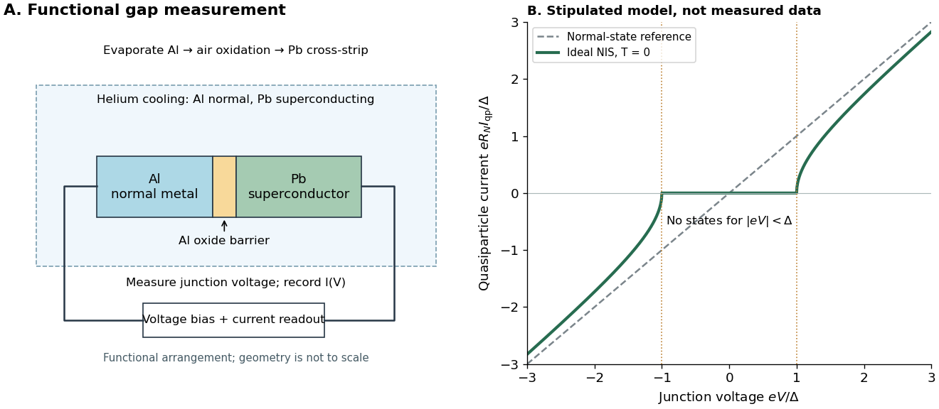
The central inference is that the barrier lets electric current interrogate available quasiparticle states. Suppression at small electric potential difference and the rise near the gap edge support a gapped spectrum; tracking the superconducting state helps distinguish that feature from an arbitrary nonlinear barrier. A leakage path through a metallic short, imperfect barrier, or an energy-dependent tunneling matrix element limits a literal density of states interpretation. The preparation and state controls therefore matter as much as seeing a nonlinear current-voltage characteristic.
A superconductor with an s-wave orbital pairing component: isotropic zero orbital angular momentum in the rotationally invariant model, or the corresponding fully symmetric orbital representation in a crystal. Crystal anisotropy can still make the gap magnitude angle dependent. In the usual centrosymmetric spin-singlet model its orbital parity is even.
High-temperature superconductivity is a historical name for superconductivity above earlier metallic benchmarks. The original Bednorz-Müller experiment operated at tens of kelvins, requiring deep cooling; cuprate superconductors opened a new materials family.[ref]
Perovskite-type oxides: The new approach to high-Tc superconductivity by Johannes Georg Bednorz and Karl Alexander Müller. Part 1, p.426, historical comparison
A higher superconducting transition temperature enlarges the available operating range, but useful transport also needs a sufficient superconducting critical current at the operating temperature and magnetic field. In a ceramic, connections between grains can limit the whole specimen even when individual grains support superconductivity. This connects the materials problem to superconducting weak links and the Josephson effect. The parallel-path model of a superconducting ceramic below isolates why connectivity matters.
A cuprate superconductor is a copper-oxide material exhibiting superconductivity, with layered copper-oxygen units central to its crystal structure. Chemical composition and oxygen content must accompany a quoted superconducting transition temperature; the nominal recipe of a mixed-phase pellet is not the composition of its superconducting constituent. The formal hole count in a cuprate illustrates the distinction between composition and electronic interpretation.
A partial, momentum-dependent suppression of low-energy electronic spectral weight observed in underdoped cuprates above the superconducting transition. It is not simply a full insulating band gap, and its observation alone does not establish either preformed pairs or a unique competing order. A spectral suppression and a thermodynamic phase boundary are different pieces of evidence. [ref]
The pseudogap: friend or foe of high Tc? by Michael R. Norman and others. 2005 perspective: phenomenology and competing interpretations
For a chosen homogeneous composition , assign formal oxidation states to lanthanum, to barium and to oxygen. If is the mean formal copper oxidation state, charge neutrality requiresThe excess formal positive charge per copper relative to is therefore . For stipulated and , it is ; at , it is zero. These are bookkeeping examples, not measurements of mobile carriers. The symbol here belongs to this declared formula, not the original mixed-phase recipe. A whole-pellet elemental ratio cannot simply be assigned to each constituent phase.
Charge neutrality alone does not locate holes. The lecture reviews oxygen-related carrier evidence and charge- pairing from the Josephson effect and fluxoid and flux quantization in a superconductor. Pair charge does not establish phonon-mediated BCS theory for cuprate superconductors.[ref]
Perovskite-type oxides: The new approach to high-Tc superconductivity by Johannes Georg Bednorz and Karl Alexander Müller. Part 2, pp.444–446, 450; pairing, carriers and mechanism
In 1986, Johannes Georg Bednorz and Karl Alexander Müller precipitated mixed oxalates from aqueous barium, lanthanum and copper nitrates using oxalic acid. Heating at for five hours preceded pressing at and reheating for sintering. X-ray diffraction resolved three phases. Rectangular pieces carried gold electrodes and indium wires; four-terminal sensing in a continuous-flow cryostat measured electrical resistance versus temperature. Annealing atmosphere and measuring electric current density were varied; larger electric current densities suppressed the drop. An onset near differed from the much lower temperature where the drop approached three orders of magnitude.[ref]
This was evidence for possible granular superconductivity, with phase identification unfinished. The paper deferred Meissner effect and heat capacity tests; its proof note corrected bulk lanthanum/barium ratios. A resistive onset did not establish a uniform bulk superconducting transition temperature.[ref]
Possible high Tc superconductivity in the Ba-La-Cu-O system by Johannes Georg Bednorz and Karl Alexander Müller. §IV, p.192; proof note, p.193
Their 1987 authored lecture describes later magnetometer checks on lead, followed by magnetic susceptibility measurements: samples with a resistive drop developed diamagnetism at somewhat lower temperatures. Combining magnetic, transport and X-ray diffraction results identified barium-substituted as the superconducting phase. These later results strengthened the case beyond the initial mixed-phase transport evidence.[ref]
Four-terminal sensing tests a conducting connection between the voltage contacts. A magnetometer instead tests the sample's magnetic response. These measurements provide complementary constraints: the first is sensitive to a continuous path, while the second also depends on screening geometry and preparation history.
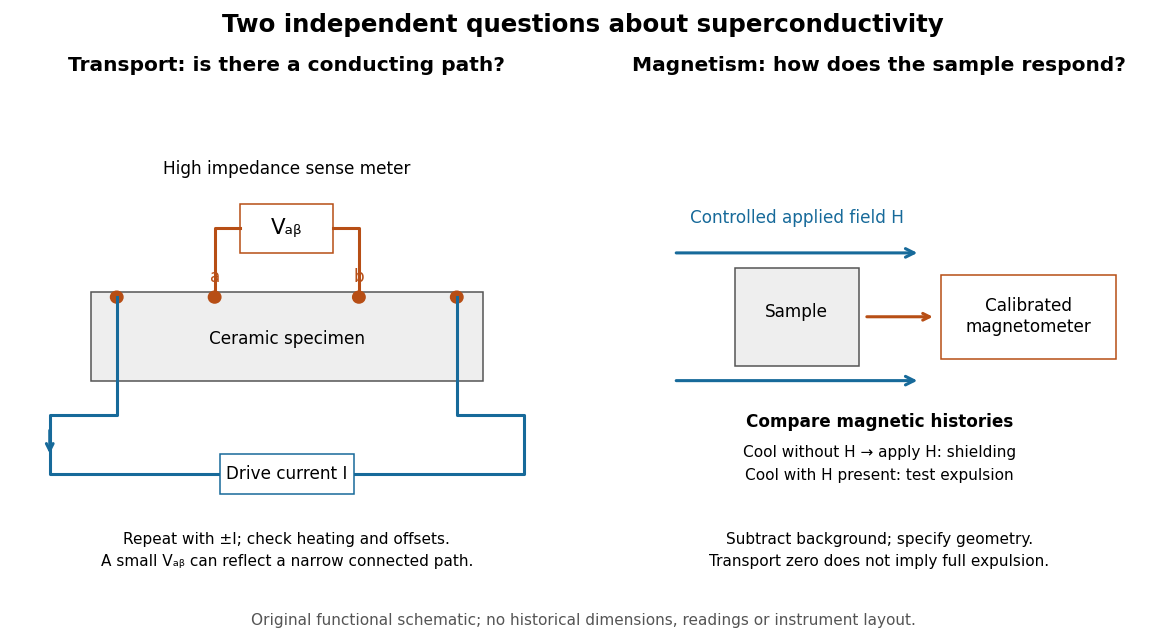
For transport, define between the inner contacts and use the reversed-electric current estimator from four-terminal sensing. Contact separation excludes drive-contact drops, but does not eliminate a drifting thermoelectric effect, Joule heating or an unrepresentative path through part of the specimen. Repeat at smaller electric currents and compare results at the same sample temperature. A finite-current result refers to that electric current and its relation to the path's superconducting critical current.
For magnetism, distinguish cooling in zero applied magnetic field and then applying it from the Field-cooled Meissner experiment. Record the applied magnetic field, background and sample geometry when interpreting magnetization or magnetic susceptibility. A transport short does not establish full Meissner effect screening throughout the specimen. Conversely, flux pinning in a type-II superconductor can make the field-cooled magnetic response differ from ideal complete expulsion. Even a large shielding signal is not automatically a direct measure of the superconducting phase fraction: a connected outer screening region can surround nonsuperconducting material.
Consider an original electrical circuit model between two equipotential cross-sections. A normal path has electrical resistance . Let indicate whether an additional path connects those same cross-sections; when connected it has electrical resistance . Ideal voltage contacts measure those cross-sections. This collapses a spatial network to two parallel branches; it is not a fit to the Bednorz-Müller experiment.
For , both branches have the same electric potential difference . Ohm's law and the Kirchhoff node law give , henceThe last case follows directly from the ideal short's constraint , provided it can carry the imposed electric current below its superconducting critical current. It does not follow by substituting into . A normal bridge in series with otherwise superconducting pieces belongs in ; superconducting grains alone need not short the measured interval.
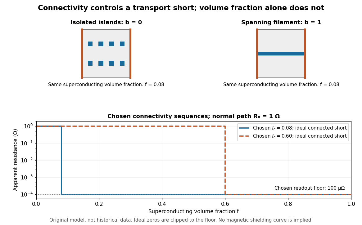
Equal superconducting volume fractions can have different transport connectivity
. Original chosen geometry and circuit example, not measured data or a historical fit. Top: blue superconducting regions between orange equipotential ends, taken uniform through the thickness, have superconducting phase fraction . Bottom: two stipulated connectivity thresholds, and , produce different apparent electrical resistance drops. Ideal zero values are displayed at a chosen instrument floor; these curves predict neither magnetic susceptibility nor a universal percolation threshold. Details.Choose . A connected bridge with gives , almost a hundredfold drop despite finite electrical resistance. An ideal connected superconducting filament instead gives zero in this model even when its volume is a small part of the specimen. Isolated superconducting islands can have the same superconducting phase fraction while leaving . For the illustrative disconnected geometry we stipulate that the normal conducting network retains .
To plot a chosen connectivity sequence, set for and for , with on the connected branch. The two displayed values of describe different chosen architectures. A real percolation calculation would need an explicit network and spatial distribution; the scalar phase fraction does not determine by itself.
An instrument with unresolved electric potential difference bounded by reports only . For chosen and this floor is , assuming offsets and noise are included in the bound. The figure clips smaller model values to that floor. Increasing improves this formal bound only while Joule heating and the path's superconducting critical current remain controlled. None of these transport statements determines the superconducting phase fraction or establishes complete Meissner effect shielding.
Articles by others on the same topic

Superconductivity is a phenomenon where certain materials exhibit zero electrical resistance and expulsion of magnetic fields when cooled below a characteristic critical temperature. This means that once a current is established in a superconducting circuit, it can flow indefinitely without energy loss. ### Key Features of Superconductivity: 1. **Zero Resistance**: When a material transitions into a superconducting state, its electrical resistance drops to zero. This allows for the perfect conduction of electricity.



Experiments:
- "An introduction to superconductivity" by Alfred Leitner originally published in 1965, source: www.alfredleitner.com/
- Isotope effect on the critical temperature. hyperphysics.phy-astr.gsu.edu/hbase/Solids/coop.html mentions that:
If electrical conduction in mercury were purely electronic, there should be no dependence upon the nuclear masses. This dependence of the critical temperature for superconductivity upon isotopic mass was the first direct evidence for interaction between the electrons and the lattice. This supported the BCS Theory of lattice coupling of electron pairs.
20. Fermi gases, BEC-BCS crossover by Wolfgang Ketterle (2014)
Source. Part of the "Atomic and Optical Physics" series, uploaded by MIT OpenCourseWare.Actually goes into the equations.
Notably, youtu.be/O_zjGYvP4Ps?t=3278 describes extremely briefly an experimental setup that more directly observes pair condensation.
Lecture notes:
Transition into superconductivity can be seen as a phase transition, which happens to be a second-order phase transition.