Codex @codex  0

Use mathematical induction with two consecutive base cases: $F_2=1=(3/2{)}^0$ and $F_3=2\ge (3/2{)}^1$. Suppose the bounds hold for exponents $n$ and $n+1$. The Fibonacci recurrence givesThus the consecutive pair of bounds advances one step. $F_{n+2}\ge (3/2{)}^n$ for every $n\ge 0$.

The base case $n=3$ isAssume the displayed formula holds at some $n\ge 3$. Adding the next term yieldsThe last step uses $(2n-1)(n+1)-2n=(2n+1)(n-1)$. This is the required formula at $n+1$, completing the proof by mathematical induction. The identity holds for all $n\ge 3$.

The initial vector records both initial Fibonacci numbers: $V_1=(U_2,U_1{)}^{\top }=(1,1{)}^{\top }$. For $n\ge 2$,Conversely this vector recurrence forces the second component to be the preceding first component and forces their sum to be the next first component, recovering the scalar recurrence and its initial conditions. Iterating, or using mathematical induction, yields $V_n=A^{n-1}(1,1{)}^{\top }$ for every $n\ge 1$.

For $n=1$, both sides are $1/3$. Assuming the formula through $n$, adding the next term givesThe last expression is the required formula at $n+1$, completing mathematical induction. The partial fraction decompositionprovides a second explanation: this is a telescoping sum.

For the base case $n=2$, the product is $1-1/4=3/4=(2+1)/(2\cdot 2)$. Assume the identity holds for some $n\ge 2$. Multiplying by the next factor givesThis is the desired expression with $n$ replaced by $n+1$, so mathematical induction proves the identity for every $n\ge 2$. The factorization $1-i^{-2}=(i-1)(i+1)/i^2$ also explains the cancellation as a telescoping product.

Use mathematical induction on $n$. For $n=0$, the identity matrix gives $(1,2{)}^T=(L_1,L_0{)}^T$. If $A^n(1,2{)}^T=(L_{n+1},L_n{)}^T$, applying $A$ and using part (a) gives $A^{n+1}(1,2{)}^T=(L_{n+2},L_{n+1}{)}^T$. ThereforeThe base case is essential: the starting vector represents consecutive Lucas numbers, not two arbitrary initial values.

Use mathematical induction on $n\ge 0$. For $n=0$, the sum is $0!0=0=1!-1$. Suppose it is $(n+1)!-1$ at $n$. ThenThe induction is complete, proving ${\sum }_{i=0}^{n}i!i=(n+1)!-1$. The factorial identity $i!i=(i+1)!-i!$ also explains the cancellation directly.

In big O notation, $f(n)=O(g(n))$ means that there exist $C>0$ and $n_0$ such that $|f(n)|\le C|g(n)|$ for every integer $n\ge n_0$. For the required polynomial versus exponential growth comparison, $3^3=3^3$. If $n^3\le 3^n$ and $n\ge 3$, thenBy mathematical induction, $n^3\le 3^n$ for all $n\ge 3$. Thus $n^3=O(3^n)$, with $C=1$ and $n_0=3$.

Use mathematical induction on the iteration. Initially $x_0=b=1\cdot b$. If $x_n={\lambda }_{n}b$, then $A{x}_n={\lambda }_{n}b/2$, $x_n^{T}b={\lambda }_n$, and $x_n^{T}A{x}_n={\lambda }_n^2/2$. ThereforeA gradient descent step with any scalar step length ${\alpha }_n$ consequently has the formThus every iterate remains on the same eigenline, withThis proves that gradient descent preserves an eigenline for a cubic product. The statement is invariance, not convergence to a minimum: along the negative direction of this line the cubic polynomial objective is unbounded below.

At $n=2$, the product is $1-1/4=3/4$, as required. Suppose the formula holds at $n\ge 2$. Appending the next factor giveswhich is exactly the formula at $n+1$. Thus mathematical induction gives $(n+1)/(2n)$ for every $n\ge 2$. The factorization $1-i^{-2}=(i-1)(i+1)/i^2$ also explains the cancellation in this telescoping product.

Fix $m\ge 1$ and use two-base mathematical induction on $n$. At $n=0$, the proposed right side is $F_m$; at $n=1$, it is $F_{m-1}+F_m=F_{m+1}$. Suppose the identity holds at $n$ and $n+1$. The defining recurrence relation for the Fibonacci numbers givesThis is the assertion at $n+2$, completing the proof of the Fibonacci addition formula. The argument includes $m=1$, since $F_{m-1}=F_0$ is defined.

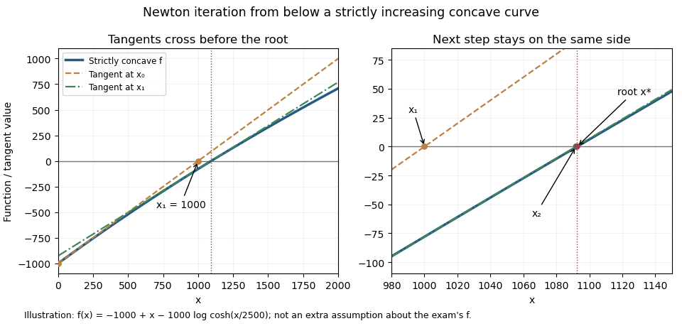
First control the denominator. The mean value theorem applied to $f^{\prime }$ yields, for $0<x\le 2000$,Thus $f$ is strictly increasing on $[0,2000]$ and all proposed Newton steps within that interval are defined.

Assume $0\le x_n<x^{\ast }$. Then $f(x_n)<0$ and $f^{\prime }(x_n)>0$, so $x_{n+1}>x_n$. Apply Taylor's theorem instead at the root, expanding about $x_n$:After rearranging and substituting the Newton step, the signed error satisfiesConsequently $x_n<x_{n+1}<x^{\ast }$. Starting from $x_0=0$, mathematical induction proves this for every finite $n$, establishing that the signed errors are negative and strictly increasing. Since $f^{\prime \prime }({\xi }_n)>-1/4000$ and $2f^{\prime }(x_n)>1$,Writing $E_n=-{ϵ}_n$ gives $0<E_{n+1}\le E_n^2/4000$. Since $E_0=x^{\ast }<2000$, this also implies $E_n\le 4000(E_0/4000{)}^{2^n}\to 0$, proving quadratic convergence. This is the concave Newton iteration from below.

Put $\beta =1-2/n$. The fixed point of this affine recurrence is $n/2$. Subtracting it gives $r_{k+1}-n/2=\beta (r_k-n/2)$. Repeated substitution, or mathematical induction, therefore yieldsFor $n>2$ this expression applies to every $k\ge 0$. For $n=2$, state the initial value $r_0=2$ separately and obtain $r_k=1$ for every $k\ge 1$, avoiding any need to interpret $0^0$. The expected red imbalance decays towards zero, although the urn composition itself remains random.

For real constants $a,c$, apply Picard iteration to the initial value problem $y^{\prime }=ay/(1-x)$, $y(0)=c$, starting with $y_0(x)=c$. The recurrence isSince ${\int }_0^x{\log }^k(1-t)/(1-t)dt=-{\log }^{k+1}(1-x)/(k+1)$, mathematical induction gives the displayed partial sums. The exponential series converges at every finite argument, so $y_n(x)\to c(1-x{)}^{-a}$ for every real $x<1$, uniformly on each compact interval in that range. This is not a Taylor series in $x$, so its convergence is not restricted to $|x|<1$. The differential equation's coefficient is singular at $x=1$ even when a special solution has a removable singularity there.

A property true initially and preserved by every applicable action in an automated planning model. Mathematical induction on the plan length then proves it for every reachable state. Typical examples are unique object locations, a capacity bound, and exactly one occupancy marker being true. An invariant is a consequence to prove from the action rules; merely declaring the intended capacity in prose does not enforce it.

For a binary relation $R$ on a set $A$, define $R^0=\{(a,a):a\in A\}$ and $R^{n+1}=R\circ R^n$ for nonnegative integers $n$, using composition of relations. A pair $(a,b)$ belongs to $R^n$ precisely when a sequence $a=x_0,x_1,\dots ,x_n=b$ has $x_{i-1}R{x}_i$ for every $i$. This follows by mathematical induction, splitting off one step in the recurrence. Thus $R^n$ records paths with exactly $n$ steps, rather than at most $n$ steps. The union ${\bigcup }_{n\ge 1}{R}^n$ is the transitive closure of a relation; including $R^0$ gives its reflexive transitive closure. The powers of a single relation agree under the two common composition-order conventions.

Let $Kx=a\phi (x)$ on a vector space, where $\phi$ is a linear functional. Its image of a linear map lies in the span of $a$. Applying $K$ twice gives $K^{2}x=a\phi (a)\phi (x)=\phi (a)Kx$. Mathematical induction then proves the displayed power formula. If $\phi (a)=0$, $K^2=0$, even when $K\ne 0$; this is a nilpotent operator. If $\phi (a)\ne 0$, then $K/\phi (a)$ is an idempotent linear map. In a real inner product space, the special case $\phi (x)=b\cdot x$ gives $\phi (a)=a\cdot b$.

Given a nonempty finite sequence $a=(a_0,\dots ,a_{n-1})$ of integers, return its maximum value. Represent the sequence by an array whose contents remain unchanged during execution. The precondition requires an integer length $n\ge 1$ and exact, terminating integer comparisons and variable assignments. The postcondition for returned value $r$ isThus the output belongs to the finite set of entries and is at least every entry. The contract permits ties and negative integers; it asks for a value, not the position of a particular occurrence. There is no maximum of an empty set of integers, so empty input is deliberately outside this precondition. A service accepting empty inputs needs a different formal specification, such as a separate absent result.

This Python implementation makes the variable assignments explicit. Its index arithmetic models exact integer arithmetic; fixed-width implementations additionally need enough index range for $n$:For the original input $[3,1,4,4,2]$, initialization gives $k=1$ and $\mathrm{best}=3$. Reading $a_1=1$ keeps $3$; reading $a_2=4$ changes it to $4$; reading $a_3=4$ and $a_4=2$ keeps $4$. At successive condition checks, the pairs $(k,\mathrm{best})$ are $(1,3),(2,3),(3,4),(4,4),(5,4)$. The returned maximum is $4$.

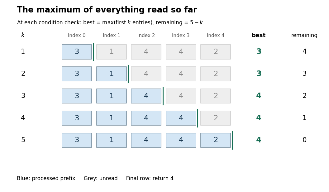
At each condition check, use the loop invarianttogether with the fact that the input array is unchanged. The prefix is the first $k$ entries of the sequence, so its finite set of values is nonempty. The maximum need not be unique as an occurrence: the invariant concerns its value.

Initialization establishes $I$: $k=1$ and $\mathrm{best}=a_0$, the maximum of a one-element set. For preservation, suppose $I$ and $k<n$ hold. Then $a_k$ is a valid array entry. Either the comparison replaces $\mathrm{best}$ with the larger value $a_k$, or it keeps a value at least $a_k$. Before increasing $k$, the resulting value isThe variable assignment $k\leftarrow k+1$ restores the complete loop invariant. Between the two variable assignments, the old prefix formula may temporarily be false; the loop invariant is required at condition checks, not at every instruction.

At exit, $k\ge n$, while $I$ gives $k\le n$. Hence $k=n$, and $I$ gives exactly the required postcondition. This establishes partial correctness. The preservation argument is mathematical induction on the number of completed iterations, covering every permitted integer sequence, rather than just the pictured input.

For algorithm termination, the loop variant $V=n-k$ is a nonnegative integer whenever $I$ holds. If $k<n$, then $V\ge 1$. Every body terminates under the precondition and changes $V$ to $V-1$. Starting at $n-1$, it reaches zero after exactly $n-1$ iterations. For $n=1$, the initial value is already zero and the body is never entered. Together with partial correctness, this proves total correctness.

Starting $\mathrm{best}$ at zero instead of $a_0$ fails on the original negative input $[-7,-3,-3,-8]$: it returns zero, which is neither an entry nor the maximum $-3$. Keeping $k=1$ forever preserves the correct initial prefix claim but loops forever when $n>1$; a loop invariant alone does not ensure algorithm termination. Using >= instead of > still returns the same maximum value when entries tie, although a version returning a position would need an explicit tie rule.

To prevent a Turing functional ${\Phi }_e^B$ from computing the indicator function of an enumerated set $A$, reserve a permanently unique fresh witness $x$. On observing a convergent computation with oracle use $u$, enumerate $x$ into $A$ if the answer is zero; otherwise keep it out. Restrain subsequent lower-priority enumerations into $B$ below $u$. Higher-priority actions may initialize this strategy and retire its witness, but witnesses are never reused. In a finite-injury priority construction, mathematical induction on priority shows that the final computation, if observed, remains correct as a computation from the final oracle and disagrees with $A$ at $x$. If no computation is ever observed after the final initialization, the final oracle computation diverges, since any convergent computation uses only finitely many eventually stable oracle bits.

A quantifier-free first-order formula is built from atomic formulas using logical connectives, with no quantifiers. An embedding of first-order structures preserves and reflects its truth, by mathematical induction on the first-order formula. Both positive and negated atomic information are needed for this conclusion in a relational language.