Picard iteration replaces a tentative trajectory by the accumulated integral of its proposed rate. For an initial value problem , , define the Picard map and its starting function byHere is the constant starting trajectory; the same symbol without its argument denotes the initial state. A fixed point of solves this integral equation, and the fundamental theorem of calculus gives the original ordinary differential equation.
For , , successive integrals giveAt , the first five values are , while . The fourth polynomial misses by about . On , every omitted term of the exponential series is nonnegative and increasing, so the largest error occurs at . The tail tends to zero, giving uniform convergence to the exponential function on this interval.
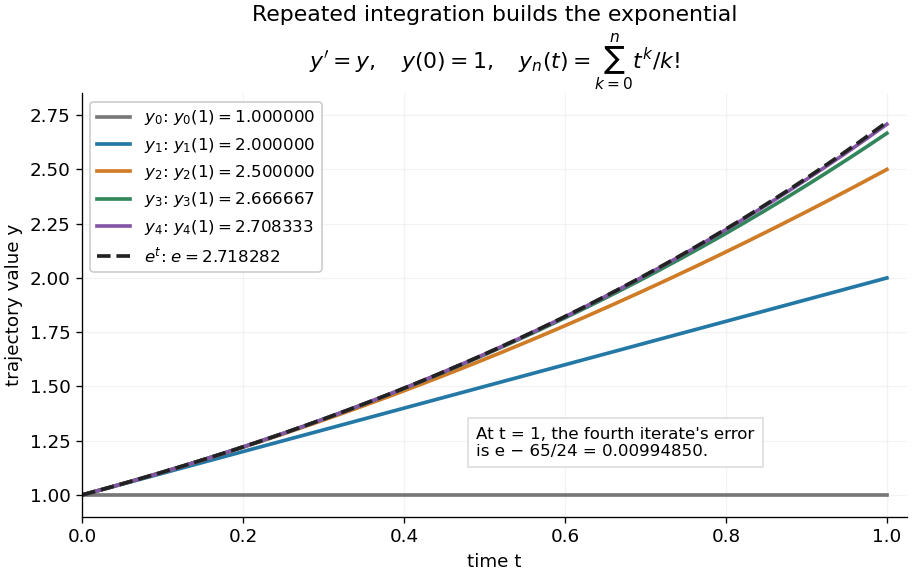
Picard iteration builds the exponential solution by repeated integration
. The first five polynomials approach the exponential function on . Endpoint values are listed in the legend; the last error is approximately . Details.
The beauty of Picard iteration is that each proposed trajectory supplies a better rate history for the next one. For this example, one integration adds exactly the next term of the exponential series. In general, the integrals may be difficult to compute, but the construction still explains local existence and uniqueness.
The short contraction mapping argument needs two independent controls. Choose a time-state cylinder on whichThe second bound is the uniform local Lipschitz condition. Set with , and . In the function space of continuous functions , use the supremum norm . On its closed ball , direct integral estimates giveThus the map preserves the closed ball and is a contraction mapping there. This closed ball is a complete metric space, so the contraction mapping theorem gives convergence to exactly one fixed point. Any other local solution of a differential equation stays in the same ball after shortening its interval, and hence agrees there.
For , take , so in the state ball and , . Choosing gives and , with the actual solution satisfying . The plotted interval is longer than this simple guarantee: the explicitly computed exponential series converges there anyway. The condition is sufficient for this one-step contraction mapping argument, rather than a necessary lifespan bound.
For real constants , apply Picard iteration to the initial value problem , , starting with . The recurrence isSince , mathematical induction gives the displayed partial sums. The exponential series converges at every finite argument, so for every real , uniformly on each compact interval in that range. This is not a Taylor series in , so its convergence is not restricted to . The differential equation's coefficient is singular at even when a special solution has a removable singularity there.
For Picard iteration , , assume and a Lipschitz constant on a rectangle containing every iterate. The first difference is at most . Integrating the preceding bound multiplied by proves the displayed estimate by mathematical induction. Its uniform bounds sum to a convergent exponential series for every finite , so the Weierstrass M-test gives uniform convergence without requiring .
For two arbitrary initial functions in a function set preserved by the Picard iteration operator , the same induction givesThus some iterate is a contraction mapping on any fixed finite interval for which every iterate stays in that set. The iterated contraction argument gives a unique fixed point of on a nonempty complete metric space, without requiring . For a rectangle with field bound and vertical radius , supplies the required self-mapping property.
Consider the Volterra integral equationwhere is continuous, , , and the continuous kernel satisfies for , with . If , there is exactly one continuous solution on the whole half-line. It is bounded, and Picard iteration beginning at converges in supremum norm with contraction ratio at most .
For a proof, the integral of the kernel is at most . Thus maps the closed ball of radius in the Banach space of bounded continuous functions into itself, since . Factoring gives on this ball. The contraction mapping theorem gives its unique fixed point. A first-exit argument shows that every continuous solution, even one not initially assumed bounded, stays strictly inside the same ball: a first time with would contradict . Reapplying the estimate gives the strict global bound , so uniqueness is unrestricted within the continuous solution class. If , zero is the only solution by the Gronwall inequality on each finite interval.
A Picard iterate is one of the successive approximate solutions of a differential equation obtained by repeatedly applying its integral solution operator. If and , the usual operator is . An integrating factor can produce a different, equivalent operator with better estimates, as in Global Picard iteration with a decaying kernel. The word iterate denotes an approximate function; Picard iteration denotes the procedure.
Articles by others on the same topic
There are currently no matching articles.