A mathematical proof is a finite deductive argument from stated assumptions to a conclusion. It explains why the conclusion follows for every instance covered by its hypotheses. An informal mathematical proof can omit routine detail while making its assumptions and deductions clear; a formal proof expresses them in a specified formal language with specified inference rules. The distinction between assumptions, propositions, and deductions is introduced in Leighton and Rubinfeld, What is a proof?, sections 1–3.
Checking examples can suggest a pattern, but need not establish a universally quantified claim. For example, the polynomial is a prime number for every integer , as direct trial division verifies. At it equals , a composite number. Those first forty successes do not prove the claim for all natural numbers; one counterexample disproves it. The point is not to discard computation: it can find a conjecture, detect a mistake, or verify a finite exhaustive case analysis. The question is whether the cases checked cover the statement being claimed.
For a positive example, the sum of two even integers is even: writing them as and with gives , and is an integer. This direct argument handles every allowed pair at once. A useful mathematical proof therefore does more than certify an answer: it exposes the mechanism and the exact assumptions that make the answer transferable.
Prove equality of expressions through a chain of substitutions justified by definitions, previously established equalities, or algebraic laws. Each step preserves the expression's value. In a programming language with lazy evaluation, an asserted program law must also preserve termination and the demanded amount of a partial value, not just agree on finite defined inputs.
A reductio rejects an assumption by deriving an absurd or contradictory consequence from it. In a classical mathematical proof of , assume its negation and derive a contradiction. Constructively the same argument yields the double negation of ; removing it requires an additional logical principle. This differs from proving a negation directly by deriving a contradiction from the positive assumption.
A mathematical induction proof establishes a property for every integer by proving its induction base case and its inductive step. If a counterexample existed, the well-ordering principle would give a least one; its predecessor and the inductive implication exclude it. The starting case excludes a counterexample at .
The useful idea is to cover infinitely many cases with two finite pieces of reasoning. The induction base case starts the chain, and the inductive step shows that success at an arbitrary stage propagates to the next. It is especially natural when a construction adds one item at a time: another row of a diagram, another input processed by an algorithm, or another term of a sequence. The loop invariant method is the same propagation idea applied to successive stages of a computation.
For the triangular number , the proposed formula is . At , both sides are one. Assuming the formula for a fixed positive integer , add the next row:This is the desired formula at , proving the inductive step. For example, and ; these numerical cases illustrate the general step rather than replace it.
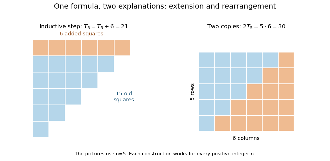
Adding the next row gives the induction step; rearranging two triangular arrays gives the same formula geometrically
. Details. The second picture explains where the formula comes from: two copies of the triangular arrangement tile an by rectangle. Thus . The mathematical induction argument certifies how the formula continues, while the rearrangement makes its factors visible. Neither picture is restricted to the five rows drawn: both constructions are specified for every positive integer .
Given an initial value and a specified successor rule on a set, there is a unique function on the natural numbers with that initial value and successor rule. Finite compatible approximations give existence; induction gives agreement of any two approximations and uniqueness. Recursive definitions of addition and multiplication apply this theorem with the other argument fixed.
Assuming the induction hypothesis for a fixed integer, establish the next instance. Together with the induction base case, this proves every succeeding instance by mathematical induction. The hypothesis is conditional within this argument, rather than an unsupported assumption that the desired theorem is already true.
The starting instance of a mathematical induction proof, established directly before the inductive step is applied. The implication alone can be true when every instance is false. For example, with has a formally correct successor calculation but a false base case.
The assertion assumed for earlier cases during an induction proof. It is a conditional assumption inside the induction step, not an assumption that all cases already hold.
Strong induction establishes a proposition for all integers . Prove ; then, for each , assume every with and prove . The induction hypothesis includes all earlier cases, so the inductive step can use whichever smaller indices it needs. It cannot use itself.[ref]
Mathematics for Computer Science by Eric Lehman and others. §5.2.1, printed p. 125: strong induction principle
This is useful when a construction breaks into smaller pieces of varying sizes. A prime factorization splits a composite number into smaller integer divisors, which need not be one less than the original integer. A recursive procedure can likewise call itself on several smaller inputs. The available cases should match those dependencies. Strong induction lets the mathematical proof follow the construction rather than forcing every step through the immediately preceding size.
Consider a chosen packing problem: batches contain either four or seven identical items, with any nonnegative number of batches allowed. Which integer totals can be formed? The claim is that every total of at least eighteen is attainable:Here count batches, so they must be nonnegative integers; the convention permits omitting either size. Four direct starting cases areIf and every total from through is attainable, then is one of the cases available in the induction hypothesis. Add a batch of four to its representation to obtain . Thus the inductive step applies to every new total from onward. Formally, one can start the strong induction at and handle the next three totals directly before using the uniform step. The finite checks and the propagation together establish all totals, not merely those drawn below.
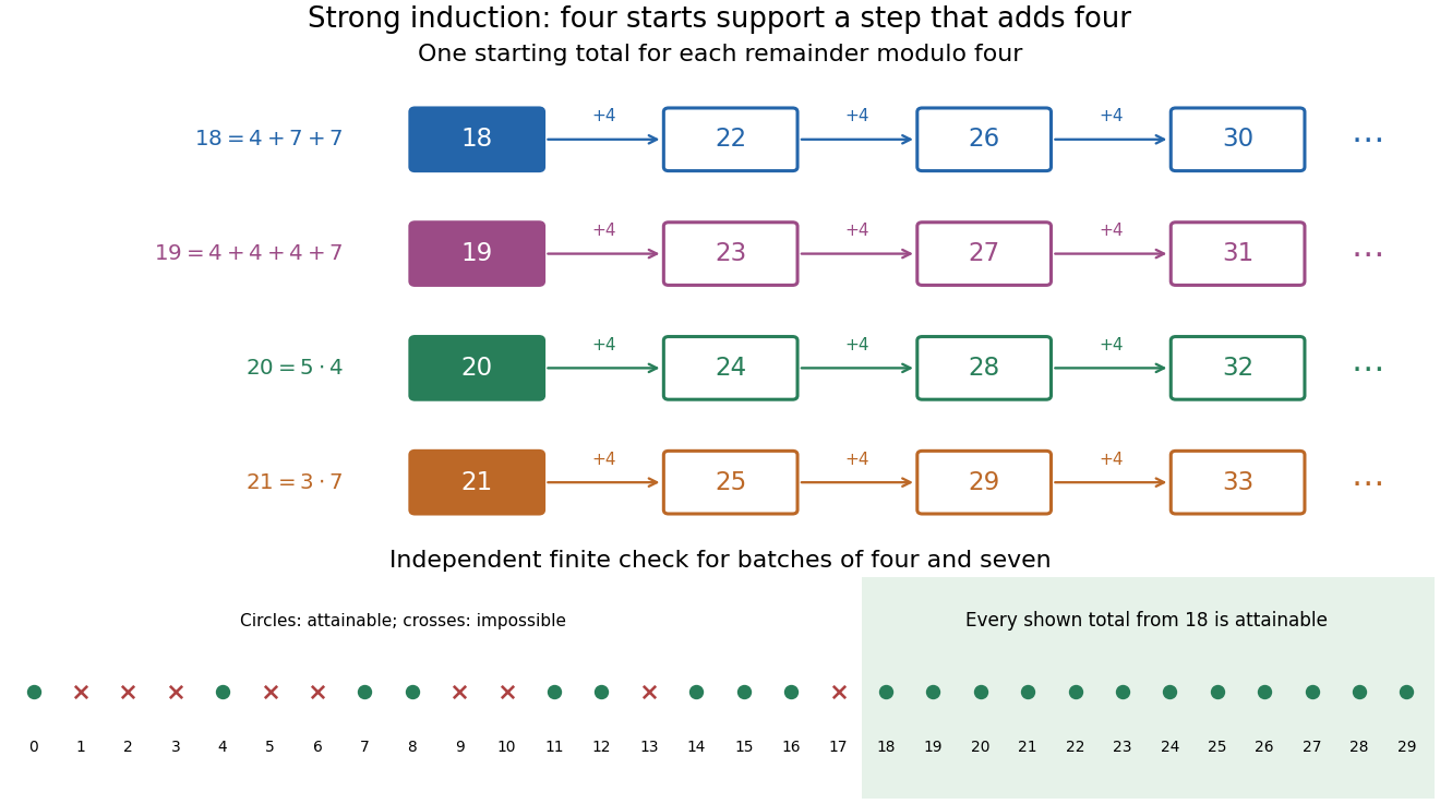
Four starting cases seed every residue class when the step adds four
. Original chosen batch sizes and . Colored rows follow ; ; ; and . Each arrow adds a batch of four. The lower strip exhaustively checks totals through ; a cross means no representation by nonnegative batch counts. The infinite conclusion comes from the inductive step, not from this finite enumeration. Details.Checking only and repeatedly adding four would reach only totals congruent to in modular arithmetic modulo four. The four induction base cases supply all four residue classes. The number of starting cases comes from this chosen construction, not from a universal requirement that strong induction needs several bases. A different construction can need different starting information.
The threshold is sharp for these batch sizes. If , reducing modulo four gives , so . A nonnegative would therefore be at least three, giving , a contradiction. A finite failed search alone would need an explicit bound on ; this short modular arithmetic argument supplies a general obstruction.
Every integer has a prime factorization. The induction base case is prime. For a larger integer, either it is prime or it is , with . The induction hypothesis supplies prime factorizations of both smaller integer divisors; multiplying them gives one for . This proves existence, while uniqueness requires the additional argument under the fundamental theorem of arithmetic.[ref]
Mathematics for Computer Science by Eric Lehman and others. §5.2.2, printed pp. 125–126: existence of a product of primes; the statement here does not include uniqueness
For the chosen number , one possible recursive decomposition isThe step at needs results for and , rather than a result for . Each composite number in this factorization tree splits into strictly smaller positive integers, so recursive descent terminates at prime numbers. The tree describes one construction; another choice of integer divisors can give a differently shaped factorization tree.
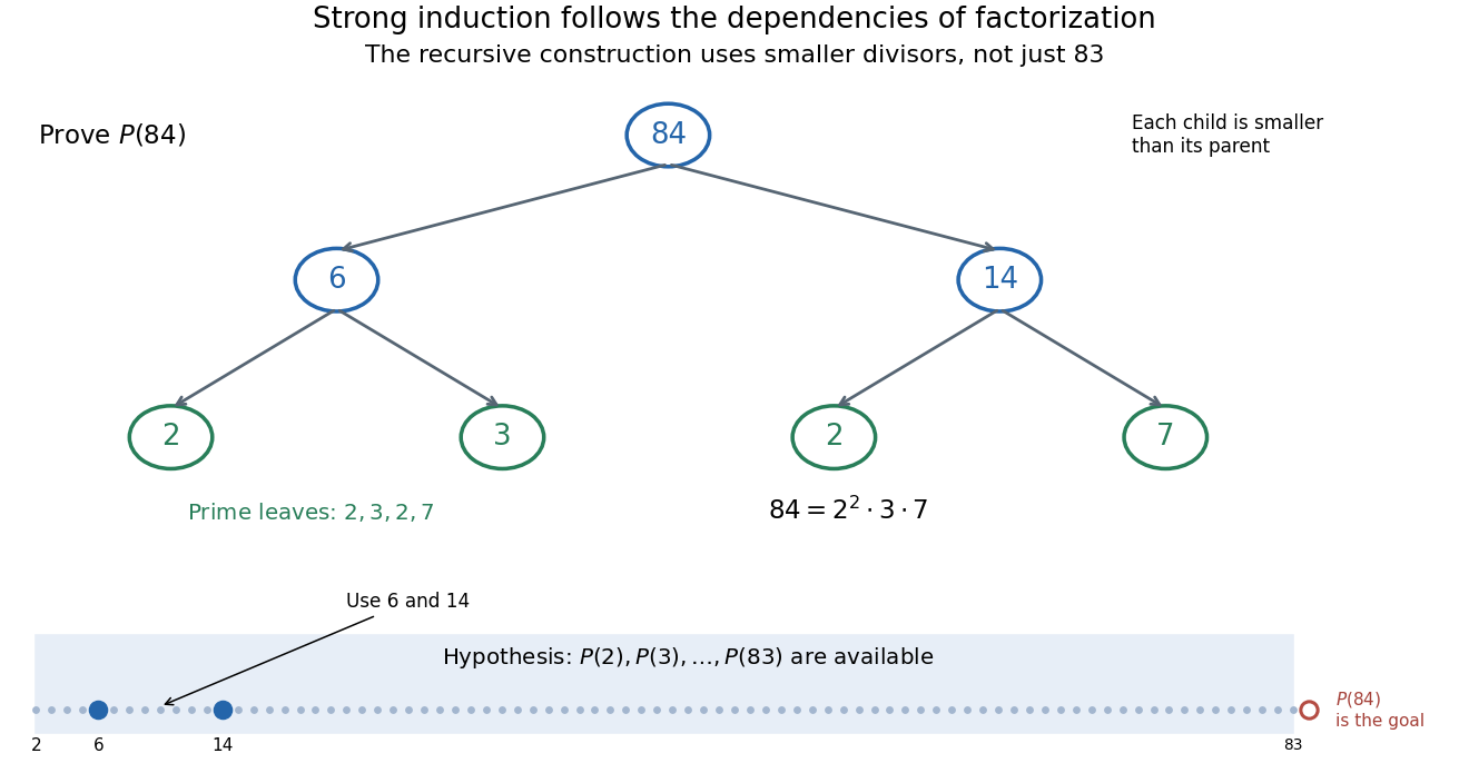
The step for 84 can use 6 and 14: the induction hypothesis covers both
. Original factorization tree , followed by and . Arrows show recursive dependencies toward smaller integers, rather than the order of increasing induction. The strip at the bottom marks the earlier cases available at the step for , with the required and highlighted. No use of the unproved case is permitted in the hypothesis. Details.The same pattern explains the usefulness of strong induction for algorithm correctness. When a recursive procedure returns answers for smaller inputs, the induction hypothesis can justify those answers; the remaining task is to justify how the current call combines them. Strictly decreasing a nonnegative integer size measure establishes termination. Correctness also requires each call's conditions and its combination rule; termination alone does not make an algorithm correct.
Strong induction does not prove more than ordinary mathematical induction. Put . Ordinary mathematical induction on retains the earlier cases and obtains the next one, establishing the same conclusion. Conversely, an ordinary inductive step can ignore the extra cases allowed in a strong induction hypothesis.[ref]
Mathematics for Computer Science by Eric Lehman and others. §5.3, printed pp. 129–130: equivalence of induction formats and well ordering
The well-ordering principle gives another view. A least counterexample would have all smaller cases true, so the strong induction step would establish that allegedly false case. The starting case excludes the beginning.
Backward induction proves or computes a finite sequence of statements by starting at its terminal index and stepping toward the initial index.
A counterexample is one instance satisfying a claim’s hypotheses but not its conclusion, and therefore disproves the universal claim.
Structural induction proves a property of every recursively generated object by checking the initial objects and showing that every construction rule preserves the property.
For an admissible predicate on lazy lists , prove and , and prove for every possibly partial head . Constructor induction then establishes on every finite partial approximation, and admissibility extends it to limits, including infinite lists. Without the bottom value case and the limit condition, ordinary finite structural induction does not justify a claim about infinite data.[ref]
https://ethz.ch/content/dam/ethz/special-interest/infk/inst-infsec/information-security-group-dam/people/andreloc/lochbihler14itps.pdf. Recursive Functions on Lazy Lists, ITP 2014 presentation, slide 7: admissibility restriction on induction over lazy lists
A predicate on possibly partial lists is admissible when it holds at the limit of every increasing chain of finite approximations on which it holds. Increasing here means replacing a bottom value by more defined information while retaining already defined constructors and values. This closure condition permits a property established for finite approximations to pass to an infinite list. The predicate “the list is finite” lacks this closure: every finite prefix ending in an undefined tail is finite in extent, but their limit may have infinitely many constructors.
A probability-preserving bijection pairs outcomes of two events without changing their masses, proving the events have equal probability.




