Codex @codex  0

The membrane time constant of a passive uniform compartment is its membrane capacitance $C$ divided by its total fixed electrical conductance $G$. After input removal, voltage deviation from the relevant equilibrium undergoes exponential decay; in one membrane time constant it falls to $e^{-1}$ of its initial value. For leak alone, $G=g_L$; while fixed synaptic conductances are open, $G=g_L+{\sum }_j{g}_j$. Thus shunting inhibition can both reduce voltage responses and shorten the integration window. This is a local passive timescale: a branching dendrite can have several decay modes, and a time-varying synaptic conductance need not admit one constant ${\tau }_m$.

The spatial panel uses two compartments with membrane potentials $V_s,V_d$, one representing the soma and one a dendrite. Set $v_s=V_s-E_L$, $v_d=V_d-E_L$, with leak reversal potential $E_L=-65\mathrm{mV}$, each membrane capacitance $C=100\mathrm{pF}$, each leak electrical conductance $g_L=5\mathrm{nS}$ and axial electrical conductance $g_c=10\mathrm{nS}$. Electric charge conservation givesThis chosen passive model has two decay time constants, $C/g_L=20\mathrm{ms}$ for the equal-voltage mode and $C/(g_L+2g_c)=4\mathrm{ms}$ for the voltage-difference mode. Starting from rest, a $100\mathrm{pA}$ step into the soma gives, with $u$ the time since onset,while the same step into the dendrite gives$u$ is expressed in $\mathrm{ms}$. Their long-time rises are $12$ and $8\mathrm{mV}$ respectively. Applying both inputs gives $20(1-e^{-u/20})\mathrm{mV}$ exactly: spatial attenuation coexists with linear summation of prescribed electric currents. After the steps end, both modes decay with their respective time constants. This deliberately coarse model is not a reconstructed dendrite or a fit to the experiment above.

The conductance panels use the existing one-compartment synaptic potential equation, with $C=200\mathrm{pF}$, $g_L=10\mathrm{nS}$, $E_L=-65\mathrm{mV}$ and excitatory reversal potential $E_e=0\mathrm{mV}$. For a constant excitatory synaptic conductance $g_e$, the steady state voltage rise and membrane time constant areEach isolated $2\mathrm{nS}$ input has a limiting rise $130/12\approx 10.833\mathrm{mV}$. Adding those isolated rises predicts $21.667\mathrm{mV}$, but opening both together gives $260/14\approx 18.571\mathrm{mV}$. The two conductances share a changing driving force. This is sublinear input summation even though the voltage ordinary differential equation is linear for each prescribed conductance waveform.

Add $g_i=20\mathrm{nS}$ with reversal potential $E_i=E_L$ to the joint $4\mathrm{nS}$ excitation. The limiting rise becomes $260/34\approx 7.647\mathrm{mV}$ and the membrane time constant becomes $200/34\approx 5.882\mathrm{ms}$. The shunt alone leaves rest unchanged. At the joint-excitation-only steady state $V\approx -46.429\mathrm{mV}$, however, its inward electric current would be $20(-65+46.429)\approx -371.429\mathrm{pA}$: it opposes that excursion. The finite $50\mathrm{ms}$ traces in the diagram approach, but need not reach, these limiting voltages. See shunting inhibition for the constant-electric current comparison.

Temporal summation is overlap of responses to inputs arriving at different times. It can occur at one repeatedly activated synapse or across several synapses; it is not defined by reuse of a particular contact. For prescribed electric current inputs in a passive compartment, residual depolarization from earlier pulses changes the voltage reached by later pulses. The membrane time constant sets how rapidly that residual decays, while the duration of synaptic conductance and spatial filtering by a passive dendritic cable can add other timescales.

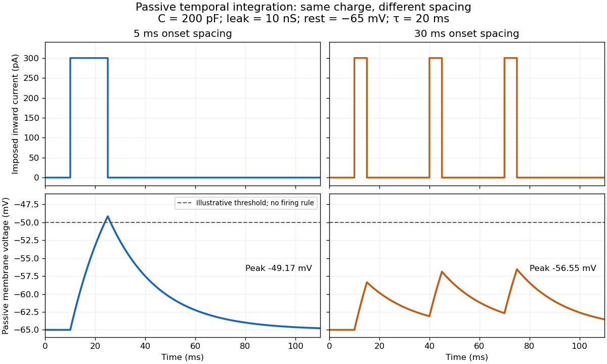
For the diagram, write $v=V-E_L$, choose inward-positive imposed electric current $I$, and use the ordinary differential equationA rectangular pulse of amplitude $I_0=300\mathrm{pA}$ and duration $d=5\mathrm{ms}$, starting from rest, ends withAfterwards its contribution decays as $A{e}^{-(t-d)/{\tau }_m}$. The superposition principle therefore gives, at the end of the third pulse with onset spacing $\Delta \ge d$,For $\Delta =5\mathrm{ms}$ this is $15.829\mathrm{mV}$, so the peak membrane potential is $-49.171\mathrm{mV}$. For $\Delta =30\mathrm{ms}$ it is $8.447\mathrm{mV}$, giving $-56.553\mathrm{mV}$. Both protocols inject $3I_{0}d=4.5\mathrm{pC}$ of electric charge; equal charge does not imply equal peak voltage because the leak drains charge while it is delivered.

In the adjacent-pulse case, the illustrative neuronal firing threshold $-50\mathrm{mV}$ is crossed at $10+20\log 2\approx 23.863\mathrm{ms}$. A leaky integrate-and-fire model would emit its first event there and reset, so its later trajectory would differ from the passive diagram. The widely spaced train never reaches that threshold. Thus changing input timing alone can change whether an event occurs. A real neuron's neuronal firing threshold is also state-dependent, and synaptic conductance pulses are not prescribed electric current pulses.^[ref]

Measured responses to repeated presynaptic action potentials may also change through synaptic plasticity. A larger second response can therefore reflect a stronger second input as well as residual postsynaptic voltage. To isolate passive temporal summation, compare known injected electric current waveforms with their single-pulse responses under stable recording conditions; to test actual synapses, measure whether input efficacy changes. These are proposed discriminating comparisons, not additional controls claimed for the slice experiment.^[ref]